

Segmentation has numerous applications in medical imaging (locating tumors, measuring tissue volumes, studying anatomy, planning surgery, etc.), self-driving cars (localizing pedestrians, other vehicles, brake lights, etc.), satellite image interpretation (buildings, roads, forests, crops), and more.
This post will introduce the segmentation task. In the first section we will discuss the difference between semantic segmentation and instance segmentation. Next, we will delve into the U-Net architecture for semantic segmentation, and overview the Mask R-CNN architecture for instance segmentation. The final section includes many example medical image segmentation applications and video segmentation applications.
The Segmentation Task

Image Source: Lin et al. 2015 Microsoft COCO: Common Objects in Context
The figure above illustrates four common image tasks:
- (a) classification, in which a model outputs the names of the classes in the image (in this case, person, sheep, and dog);
- (b) object localization, more commonly called “object detection” in which a model outputs bounding box coordinates for each object in the image;
- (c) semantic segmentation, in which the model assigns an object category label to each pixel in the image. In this example, sheep pixels are colored blue, dog pixels are colored red, human pixels are teal, and background pixels are green. Notice that although there are multiple sheep in the image, they all share the same label.
- (d) instance segmentation, in which the model assigns an “individual object” label to each pixel in the image. In this example, the pixels for each individual sheep are labeled separately. Instead of having a generic “sheep” pixel class, we now have five classes for the five sheep shown: sheep1, sheep2, sheep3, sheep4, and sheep5.
Here is another illustration of the difference between semantic segmentation and instance segmentation, showing how in semantic segmentation all “chair” pixels have the same label, while in instance segmentation the model has identified specific chairs:

Image Source: StackExchange
Here is an application of both semantic segmentation and instance segmentation to algae images:

Image Source: Ruiz-Santaquiteria et al. 2020 Semantic vs. instance segmentation in microscopic algae detection.
The following images show model predictions for instance segmentation:

Image Source: Chen et al. MaskLab: Instance Segmentation by Refining Object Detection with Semantic and Direction Features.
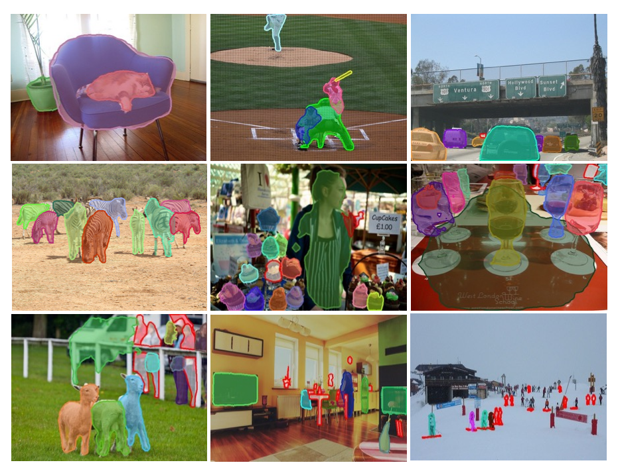
Image Source: Pinheiro et al. 2015 Learning to segment object candidates.
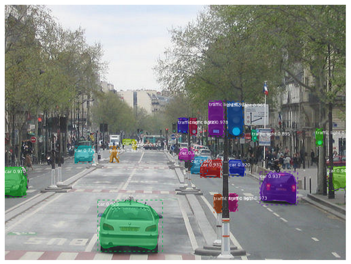
Image Source: matterport/Mask_RCNN
U-Net: Convolutional Networks for Biomedical Image Segmentation
The U-Net paper (available here: Ronneberger et al. 2015) introduces a semantic segmentation model architecture that has become very popular, with over 10,000 citations (fifty different follow-up papers are listed in this repository). It was initially presented in the context of biomedical images but has since been applied to natural images as well.
The U-Net is a type of convolutional neural network (CNN). If you would like an introduction to neural networks, please see this post. For an introduction to CNNs, please see this post. Finally, for a short history of CNNs, you can check out this post.
The basic idea of the U-Net is to perform the following task:
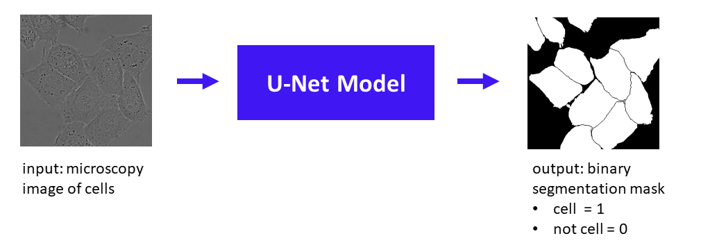
Cell/Mask Image Source: Ronneberger et al. 2015
Given an input image, in this case a grayscale microscopy image of cells, the U-Net model produces a binary mask of 1s and 0s, where 1 indicates a cell and 0 indicates background (including borders between cells). Note that this is a semantic segmentation task because all cells receive the same label of “cell” (i.e. we don’t have different labels to distinguish between different individual cells, as we would for instance segmentation.)
This schematic shows the setup of training a U-Net model:

Before the model is fully trained, for a given input image it will produce a binary segmentation mask that has problems, e.g. the “predicted binary segmentation mask” shown in the figure above, where some cells are missing or have incorrect borders. The U-Net loss function compares the predicted mask with the ground-truth mask, to enable parameter updates that will allow the model to perform a better segmentation on the next training example.
Here is the U-Net architecture:
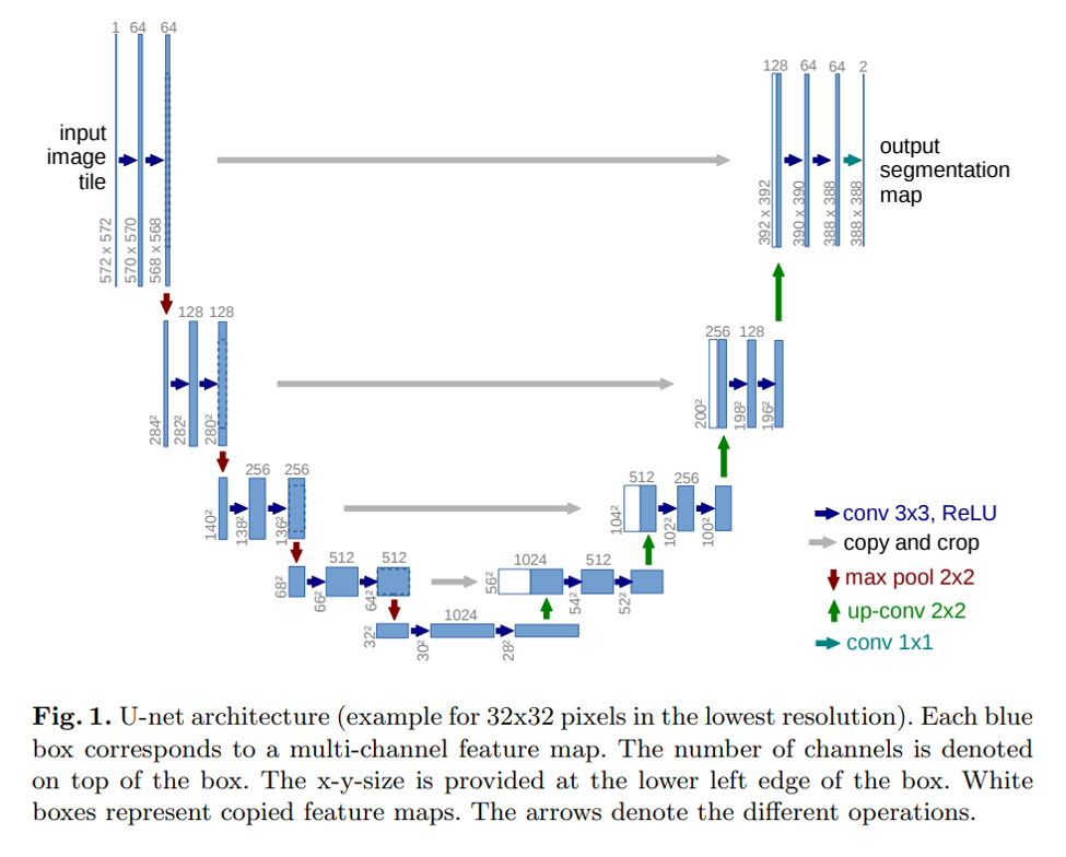
Figure 1. of Ronneberger et al. 2015
From this figure, the name “U-Net” is apparent, as the architecture diagram shows a U shape. The basic idea of the U-Net is to first obtain a lower-dimensional representation of the image through a traditional convolutional neural network, and then upsample that low-dimensional representation to produce the final output segmentation map.
It’s helpful to use the architecture diagram key provided in the lower right-hand corner, which explains what operations each arrow type corresponds to:

The U-Net consists of a “contracting path” and an “expansive path”:
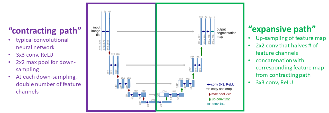
Modified from Figure 1. of Ronneberger et al. 2015
The “contracting path” is a traditional CNN, which produces the low-dimensional representation. The “expansive path” up-samples the representation to produce the final output segmentation map. Gray arrows represent copying operations, in which high-resolution feature maps from the “contracting path” are copied over and concatenated to feature maps in the “expansive path” to make it easier for the network to learn a high-resolution segmentation.
The U-Net does not have any fully connected layers, meaning the U-Net is a fully convolutional network.
Producing the Predicted Segmentation Map: 1 x 1 Convolution and Pixel-Wise Softmax
At the last layer of the U-Net a 1 x 1 convolution is applied to map each 64-channel feature vector to the desired number of classes, which in the paper is considered to be two classes (cell/background). If you want to use the U-Net for semantic segmentation with several classes, e.g. 6 classes (dog, cat, bird, turtle, cow, background) then the 64-channel feature vector can be mapped to 6 classes (6 channels) instead.
Here is a close-up from Figure 1 showing the very last part of the “expansive path” where a 64-channel feature vector is produced by a [conv 3×3, ReLU] operation, and is finally mapped to a 2-channel feature vector (cell vs. background) using a teal-colored arrow representing a 1 x 1 convolution:
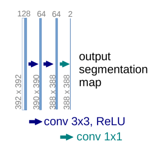
Modified from Fig. 1 of Ronneberger et al. 2015
A pixel-wise softmax is applied to the final [2-channel, 388 height, 388 width] representation to obtain the final output, a predicted segmentation map.
The pixel-wise softmax function is:
![]()
For more details on the softmax function, see this post.
The pixel-wise softmax can be conceptualized as follows. Think of the output map as a 388 x 388 image. Each pixel in that image is represented by K values, one value for each of the K channels, where K is the number of classes of interest. For each pixel we take a softmax over the K channels so that one channel will “stick out” as the highest value; this highest channel determines the class assigned to that pixel.
U-Net Weighted Cross-Entropy Loss
The U-Net is trained using a cross-entropy loss:
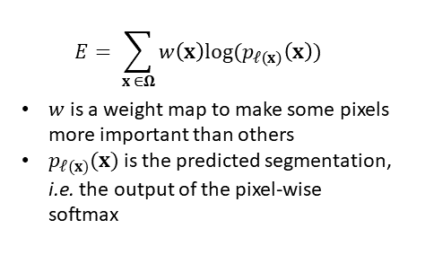
This is a typical cross-entropy loss, with the addition of the weighting w(x) which provides a weighting to tell the model that some pixels are more important than others.
The weight map w is pre-computed based off of each ground truth segmentation using traditional computer vision techniques. Specifically, morphological image processing is applied to the ground truth segmentation to identify the thin borders that separate cells, and then the weight map is created so that these thin borders separating cells are given high weights. Incorporating this weight map into the cross-entropy loss means that the U-Net will be heavily penalized if it leaves out these thin borders between cells or if it draws them in the wrong place. The overall goal of using the weight map in the loss is to “force the network to learn the small separation borders […] between touching cells.”
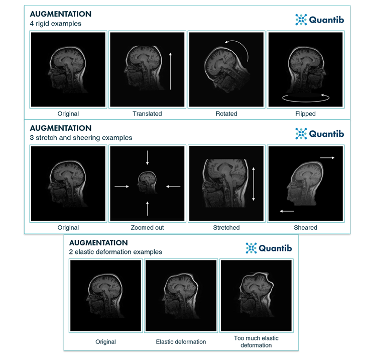
U-Net Data Augmentation
Building a dataset to train a segmentation model is time-consuming due to the need to hand-draw correct ground-truth segmentations. Accordingly, the size of the final data set may be small. In the U-Net paper the authors employ data augmentation to increase the effective size of the training data. They apply random shifts, rotations, gray value variations, and random elastic deformations to the training samples. Elastic deformations can be especially useful in medical images because (to put it colloquially) biological samples are often “squishy” meaning that the outputs of the elastic deformations are still “realistic.”
Here are some examples of data augmentation applied to a brain image, from the Quantib blog:
Overall, at the time of publication the U-Net model achieved state-of-the-art results on cell semantic segmentation tasks, and was subsequently used for a wide variety of natural image and medical image segmentation applications.
Mask R-CNN for Instance Segmentation
What about instance segmentation? Recall that in instance segmentation, we don’t just want to identify cell vs. background pixels – we want to separate individual cells. One model that can perform the instance segmentation task is Mask R-CNN. Mask R-CNN is an extension of the popular Faster R-CNN object detection model.
The full details of Mask R-CNN would require an entire post. This is a quick summary of the idea behind Mask R-CNN, to provide a flavor for how instance segmentation can be accomplished.
In the first part of Mask R-CNN, Regions of Interest (RoIs) are selected. An RoI is a patch of the input image that contains an object with high probability. Multiple RoIs are identified for each input image.
In the second part of Mask R-CNN, shown in the figure below, each RoI is used to obtain three model outputs:
- the final predicted class for this RoI (the category of the object, e.g. “person”)
- the final predicted bounding box obtained from this RoI (coordinates for the bounding box corners, which provides basic object localization)
- the final predicted segmentation (e.g. silhouette of the person, which provides highly detailed object localization)
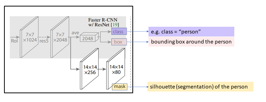
Image modified from He et al. 2018 Mask R-CNN
An RoI is considered “positive” if it overlaps enough with a ground-truth bounding box. The Mask R-CNN includes a mask loss, which quantifies how well the predicted segmentation masks match up with ground truth segmentation masks. The mask loss is only defined for positive RoIs – in other words, the mask loss is only defined when the relevant RoI overlaps enough with a true object in the image.
After it is trained, the Mask R-CNN can produce class, bounding box, and segmentation mask annotations simultaneously for a single input image:
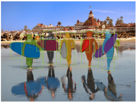
Image Source: He et al. 2018 Mask R-CNN
Mask R-CNN can also be used for keypoint detection. In the example below, the keypoints are visualized as dots connected by lines:
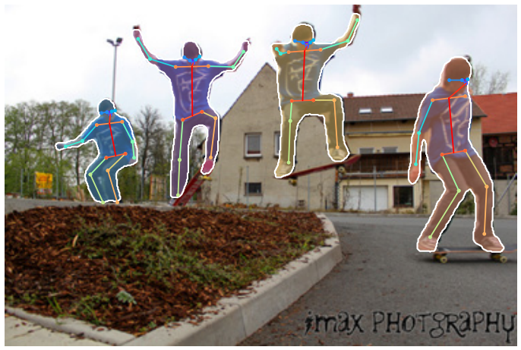
Image Source: He et al. 2018 Mask R-CNN
Creating a Data Set to Train An Instance Segmentation Model
It’s interesting to consider how much work goes in to creating data sets appropriate for training instance segmentation models. One popular instance segmentation data set is MS COCO, which includes 328,000 instance-segmented images. MS COCO was created in three stages:
- Category labeling: Mark a single instance of each object category per image. 8 workers per image. 91 possible categories. 20,000 worker hours.
- Instance spotting: Mark every instance of every object with an “X.” 8 workers per image. 10,000 worker hours.
- Instance segmentation: Perform segmentation of every instance, i.e. trace the outlines of all object instances manually. Each image was segmented by 1 trained worker and checked by 3 – 5 other workers. 55,000 worker hours.
In total, that’s 85,000 worker hours, which is equivalent to one person working 7 days a week, 12 hours a day, for over NINETEEN YEARS!
If you are interested in exploring instance segmentation further, the COCO data set can be downloaded here.
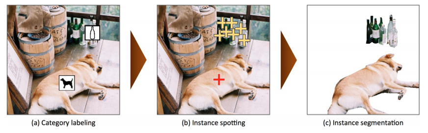
Image Source: Lin et al. 2015 Microsoft COCO: Common Objects in Context.
Medical Image Segmentation
Here is a sampling of some cool applications of segmentation in medical imaging.
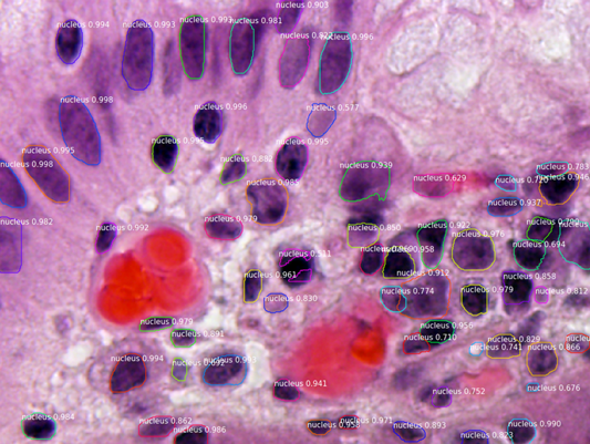
Segmenting the nuclei of cells (darker purple.) Source: matterport/Mask_RCNN, Segmenting Nuclei in Microscopy Images
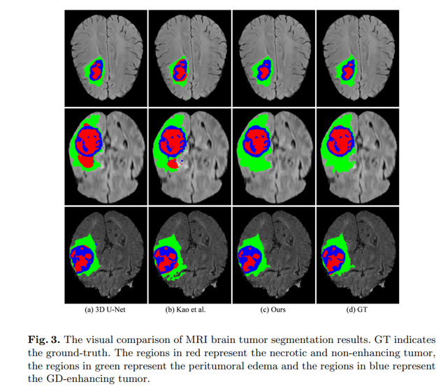
Segmenting brain tumors in MRI scans. Source: Chen et al. 2019 3D Dilated Multi-Fiber Network for Real-time Brain Tumor Segmentation in MRI.
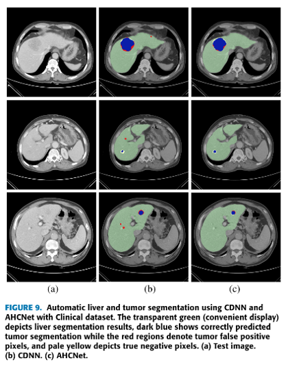
Segmenting liver and tumor in CTs. Source: Jiang et al. 2019 AHCNet: An Application of Attention Mechanism and Hybrid Connection for Liver Tumor Segmentation in CT Volumes
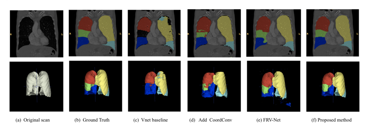
Segmenting the different lobes of the lung (right upper lobe, right middle lobe, right lower lobe, left upper lobe, lingula, left lower lobe). Source: Wang et al. 2019 Automated segmentation of pulmonary lobes using coordination-guided deep neural networks.
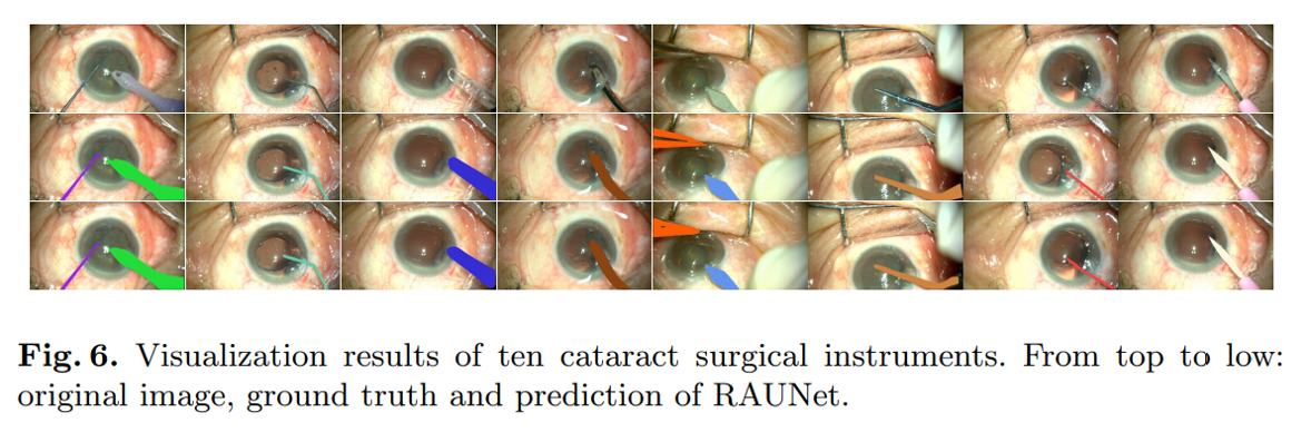
Segmenting cataract surgery instruments. Source: Ni et al. RAUNet: Residual Attention U-Net for Semantic Segmentation of Cataract Surgical Instruments.
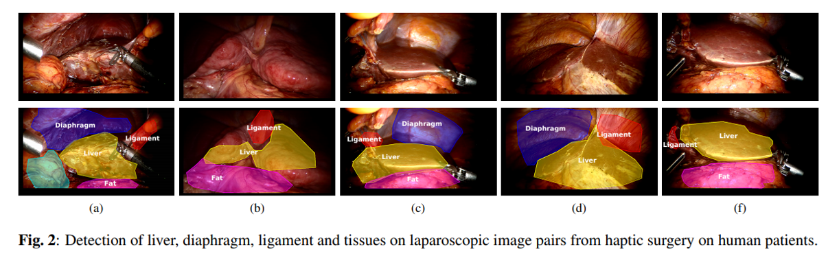
Segmenting multiple organs on laparoscopic surgery images. Source: Haouchine et al. 2016 Segmentation and Labelling of Intra-operative Laparoscopic Images using Structure from Point Cloud.
Video Segmentation Examples
It’s also possible to apply segmentation algorithms to videos! Here are two neat examples:
GIF Source: matterport/Mask_RCNN. To watch the full 30-minute video, see Mask RCNN – COCO – instance segmentation by Karol Majek.
Segmenting surgical robot. Source: matterport/Mask_RCNN
Summary
- In semantic segmentation, each pixel is assigned to an object category;
- In instance segmentation, each pixel is assigned to an individual object;
- The U-Net architecture can be used for semantic segmentation;
- The Mask R-CNN architecture can be used for instance segmentation.
About the Featured Image
The featured image is from the Mask R-CNN paper: He et al. 2018 Mask R-CNN.
As an independent researcher (MD + AI PhD + 7 yrs prior founder/CEO experience), I build and evaluate cutting-edge healthcare AI for startups. Contact me to learn more.
Want to be the first to hear about my articles bridging healthcare, artificial intelligence, and business—and get a free list of my favorite health AI resources? Sign up here.

Comments are closed.