Introduction to Neural Networks

What are neural networks?

To quote the repository of all human knowledge, “artificial neural networks […] are computing systems vaguely inspired by the biological neural networks that constitute animal brains.”

Biological neurons and “neurons” in artificial neural networks both take in signals from other neurons and produce some output accordingly. The power of both kinds of neural networks comes not from a single neuron acting alone, but from the cumulative effect of many neurons together. But the similarities stop there. A biological neuron contains immensely complex molecular machinery, and an artificial neural network neuron encompasses a few simple math operations.

Artificial neural networks have been successfully applied to images, audio, text, and medical data. This post will introduce you to how artificial neural networks compute.

Overview

Let’s say you want to build a model that predicts a patient’s hospital admission risk based on their medical record. You could assign numeric values to different components of a medical record to build a risk model, e.g. you could weight a diagnosis of diabetes as a “2”, a diagnosis of influenza as a “1.5”, and a diagnosis of stage 4 lung cancer as a “10” for a “model equation” of:

2*diabetes + 1.5*influenza + 10*cancer = risk.

For example, Fred has diabetes and the flu, but not cancer, so his risk would be (2*1) + (1.5*1)+ (10*0) = 3.5.

But how do you know what weight each of the diagnoses should have (i.e., what coefficients to use in this equation)? Should diabetes actually have a weight of 2? Maybe the weight should be 1.63, or 6, or 0.0001.

This is where machine learning methods can be helpful. In supervised machine learning, you provide a model with input/output pairs (for example, input = Fred’s medical history, output = whether Fred went to the hospital), and the model learns what weights to assign to each piece of the input in order to best predict the desired output. In other words the model figures out how important or unimportant each of the input pieces is (different diagnoses) is for predicting the output (future hospital admission).

There are many kinds of neural networks. The simplest kind of neural network is a feedforward neural network, meaning that information only flows forwards through the neurons. For the remainder of this post I will describe supervised learning with feedforward neural networks.

Data

If you want to predict a patient’s risk of hospital admission, you could extract diagnoses, procedures, medications, and lab values from that patient’s medical record (input “X”), and then check whether that patient was later admitted to the hospital (output “y”, the true answer). You want to use “X” to predict “y”, i.e. use their medical record to predict whether they will go to the hospital or not. You also want many training examples – i.e. you want thousands of example patients, not just one.

Anatomy of a feedforward neural network

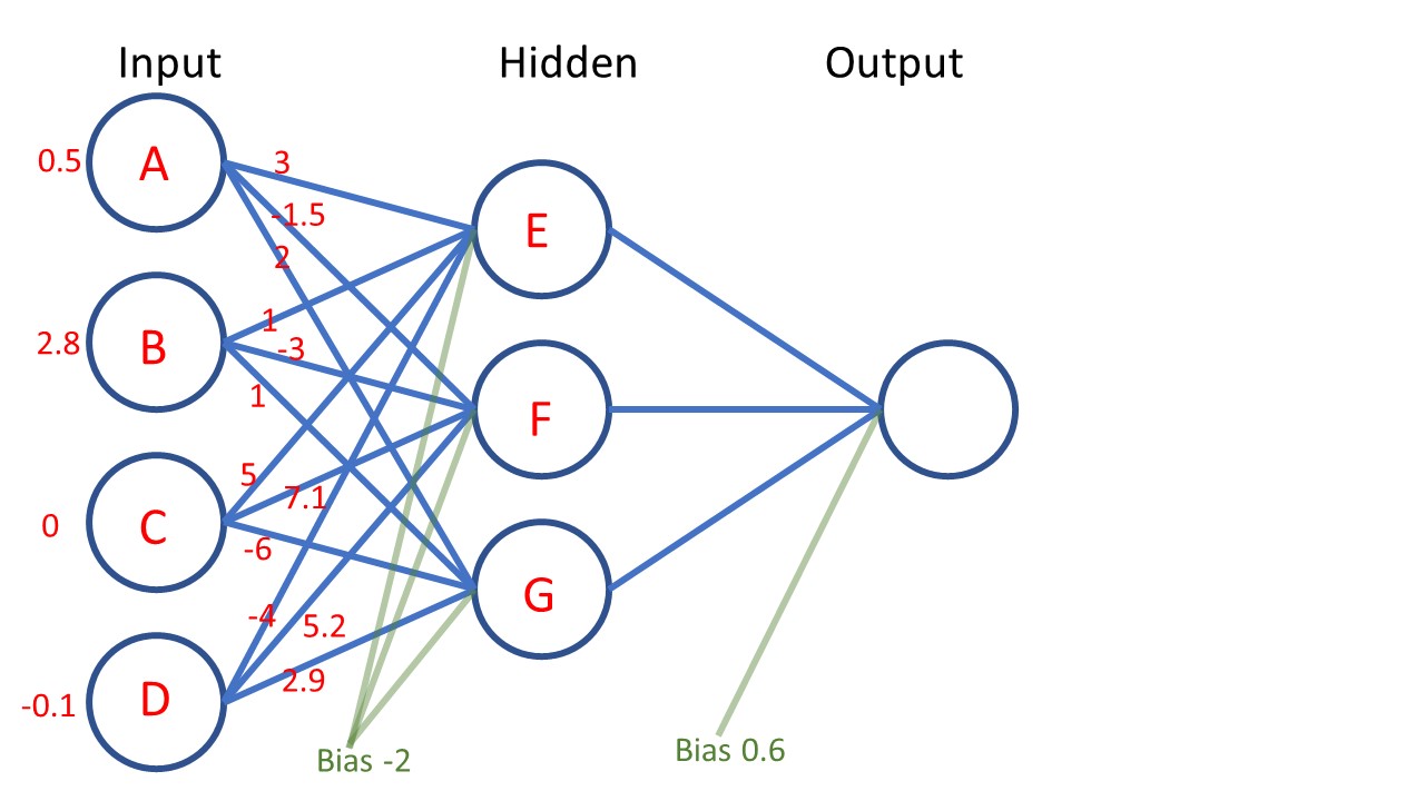
This neural network has three layers: an input layer, a hidden layer, and an output layer. Everything in between the input and the output is referred to as a “hidden layer.” You could build a neural network that has hundreds of hidden layers if you wanted to.

The input layer simply takes in a single example of the input data: for instance, the pieces of a single patient’s medical record. Here, the raw input values from top to bottom are shown in red as 0.5, 2.8, 0, and -0.1, corresponding to input neurons that I’ve labeled A, B, C, and D. These input values have a meaning. The meaning is different depending on what problem you are solving and what data you are using. Perhaps here, inputs A, B, and C are particular lab values, and D is percent change in weight over the past year (e.g. -0.1 means the patient lost 10% of their weight in the past year.)

The inputs can be any positive or negative number. Generally, the raw values are “normalized” to squash the values to be small, because neural networks have a harder time learning if some of the inputs are huge (for example 183 cm of height) and some of the inputs are tiny (for example 0.6 mg/dL creatinine.)

The hidden layer can be thought of as capturing some intermediate values in the neural network’s calculations. If you hear people talking about a “hidden representation” of the input data (or the “latent space”) they are often referring to hidden layers of a neural network. In this picture, the “latent space” is 3-dimensional because there are 3 hidden neurons: E, F, and G. If you made a neural network that had 300 hidden neurons, you could say there was a “300-dimensional latent space.” The point is that the hidden layer captures some intermediate numerical representation that is partway between the input and the output.

The output layer puts out the final answer. Here, there is only one output neuron shown. Perhaps this output node produces a probability of hospital admission. You can also have multiple output nodes, if you want to predict many different things at the same time. For example, you might have two output nodes: one to predict risk of hospital admission and another to predict mortality.

Weights: The blue lines connecting the neurons are the weights of the neural network. They represent multiplication operations. I’ve written out some values for the first weights in red. Note that example values for the weights leading to the output layer are not written out in this figure. A weight of value “3” connecting node A to node E indicates that you take the value currently inside of node A, multiply it by 3, and use the result as a component of the value for node E.

Bias: The green lines labeled “bias” are the biases of the neural network. They represent addition operations. A bias of value “6” applied to a node means that you take the value of that node and add “6” to it.

The most important difference between weights and biases is that weights indicate multiplication, and biases indicate addition.

The “learning” part of “machine learning” refers to the algorithms used to figure out good settings of the weights and biases. The weights and biases are “trainable parameters” because we use the process of neural network training to figure out good values for the weights and biases.

Where does the network structure come from?

When you are designing a neural network, you choose the structure.

You choose the size of the input layer based on the size of your data. If you data contains 100 pieces of information per example, then your input layer will have 100 nodes. If you data contains 56,123 pieces of data per example, then your input layer will have 56,123 nodes.

You also choose the number of hidden layers, and the number of nodes within each of those hidden layers. Usually a good rule of thumb is that there should not be a radical difference between the number of nodes in your input layer and the number of nodes in your hidden layer. For example, you don’t want an input size of 300,000 and a hidden layer size of 2, because that will result in throwing away a lot of information. Some neural networks have hundreds of hidden layers, but it is possible to solve many interesting problems using neural networks that have only 1 or 2 hidden layers.

You choose the size of the output layer based on what you want to predict. If you want to predict the risk of diabetes, you would have 1 output node. If you want to predict the risk of 10 diseases, you would have 10 output nodes.

Training the network

Training a neural network involves looking at all of the training examples in the data set, to learn good values of the weights and biases. Training can be broken down into specific steps:

(1) Initialization: choose random numbers for each of the weights and biases in the model. At this point the model doesn’t know anything.

(Note: In practice, the random initialization of the weights is not completely random. You’re not going to initialize one weight to 99,003 and another to 0.000004. Setting up the random initialization in a principled way helps a lot with successful neural network training. One popular weight initialization method is called “Glorot” or “Xavier” initialization. Each weight is set to a small random number, for example between -0.01 and +0.01. This number is drawn from a normal distribution with zero mean and a variance based on the neural network structure.)

(2) Forward pass: Give the neural network one training example: for instance, input “X” may be data from an individual patient’s medical record, and the corresponding correct answer “y” may be whether or not that individual patient was later admitted to the hospital. The neural network will use the randomly-initialized weights to compute its own answer for this training example. The neural network’s answer is most likely NOT going to match the correct answer “y”, because the neural network hasn’t learned anything yet.

(2) Backward pass: Quantify how wrong your network was on the example you just gave it. This involves a “loss function” – for example, [output answer  – correct answer]² (which is a squared error loss). If your network computed “0.4” as its output answer, but the correct answer was 1 (i.e. the patient was admitted to the hospital), then the loss would be [0.4  – 1]² = 0.36.

Once you know the loss, you compute derivatives across all the weights of the neural network to tell you how to tweak the weights so that the neural network will be less wrong the next time around. Recall from calculus that the derivative can be thought of as measuring the slope at a particular place on a curve. The slope we care about here is the slope of the loss function, since the loss function tells us how wrong we are. We want to know how to go “down the slope” – i.e., how to travel “downhill” to make our loss function smaller. Calculating the derivatives (the slopes) tells us how to push each of the weights in the right direction to make the neural network less wrong in the future.

Notes: (a) if you are using a popular machine learning framework like Tensorflow, you don’t actually calculate any derivatives yourself – calculation of derivatives is already built into the software. (b) In most other online resources about backpropagation, the derivative is typically referred to as the “gradient.” A “gradient” is just a multivariable derivative.

The method is called “backpropagation” because you are “propagating the error back” through your entire neural network to figure out how to make the neural network better. Each of the weights and biases will be slightly modified before the next forward pass/backward pass.

(3) Repeat the forward pass and the backward pass for many thousands of training examples. With each training example, the weights of the neural network get a little bit better. Eventually, with enough training examples, the neural network gets really good at using the inputs to predict the outputs, and you have a useful model!

Detailed Example: Forward Pass

Here is a detailed example of the forward pass, where the neural network computes an answer using some input data.

The figure above shows all of the weights leading to hidden node E highlighted in gold. The current values of the weights from top to bottom are 3, 1, 5, and -4. On the bottom right, you can see how the value fed into node E is computed. You take the input value of 0.5 (corresponding to input node A) and you multiply it by the weight that links input node A and hidden node E, which in this case has value 3. You take the input value of 2.8 (corresponding to input node B) and you multiply it by the weight that links input node B and hidden node E. You do this for all of the input nodes and sum the results together: (0.5 from node A)(3 from A-E weight) +  (2.8 from node B)(1 from B-E weight) + (0 from node C)(5 from C-E weight) + (-0.1 from node D)(-4 from D-E weight) = 4.7.

What about the green lines for the “bias”? Recall that bias signifies addition. The bias value assigned to this layer is -2. That means we subtract 2 from the value we just calculated: 4.7 – 2 = 2.7. The value 2.7 is thus our final value that we feed to hidden node E.

In the figure above, the weights leading to hidden node F are all highlighted in gold. The values of these weights from top to bottom are -1.5, -3, 7.1, and 5.2. We perform the same calculations as before: (a) Multiply the input values (red) with the corresponding weight value (gold); (b) sum these together; (c) add the bias term (green).

In the figure above, we see the weights leading to hidden node G highlighted in gold, as well as the calculation of the value fed to node G.

Nonlinearity

So far, we have only done multiplication and addition operations. However, using only multiplication and addition limits the kinds of transformations we can do from the input to the output. We are assuming that the relationship between the input and the output is linear. When modeling the real world, it’s nice to have more flexibility, because the true relationship between the input and the output might be nonlinear. How can we allow the neural network to represent a nonlinear function?

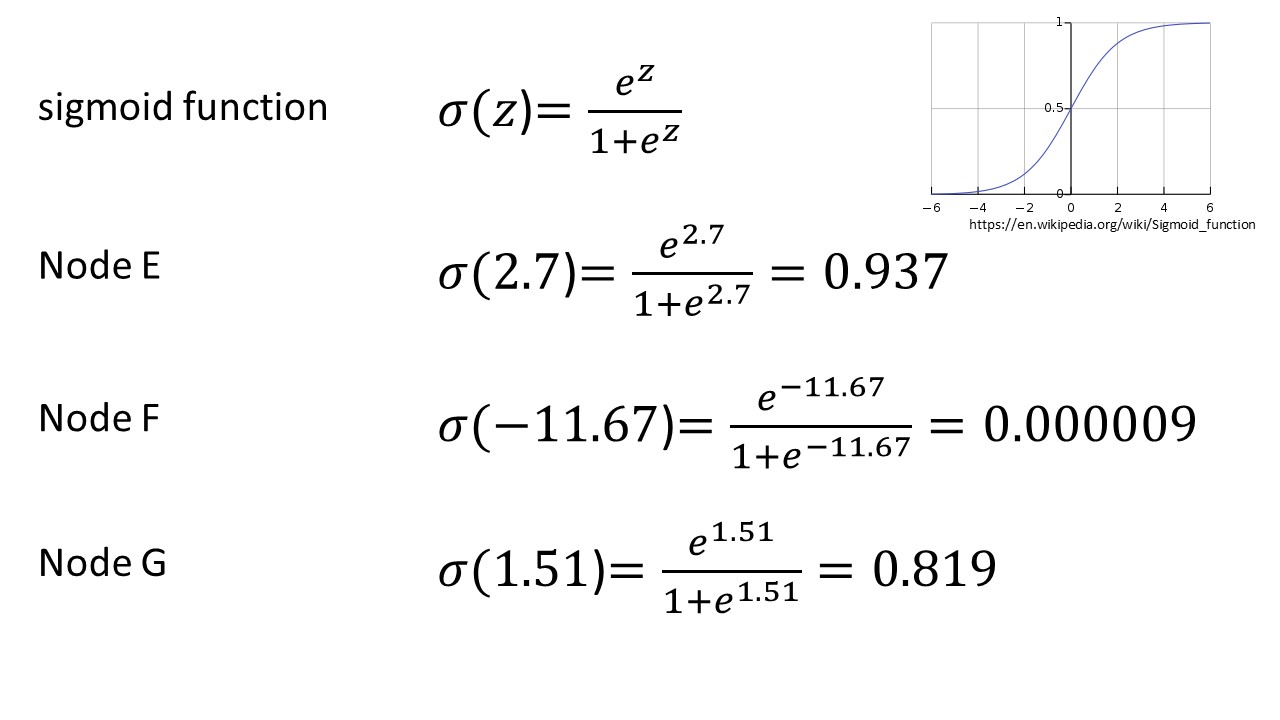
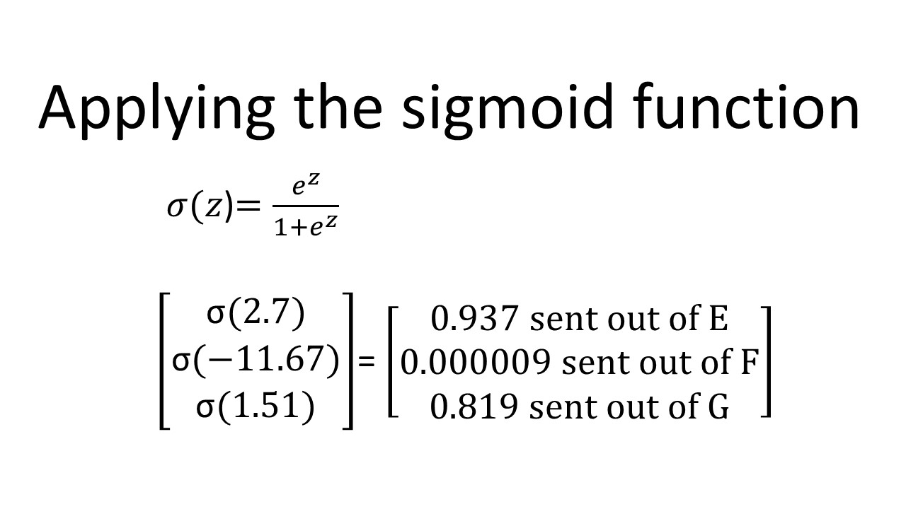
We add in “nonlinearities”: each neuron applies a nonlinear function to the value it receives. One popular choice is the sigmoid function. So, here, node E would apply the sigmoid function to 2.7, node F would apply the sigmoid function to -11.67, and node G would apply the sigmoid function to 1.51.

This is the sigmoid function:

Key points:

(1) the sigmoid function is not linear, which helps the neural network learn more complicated relationships between the input and output

(b) the sigmoid function squashes its input values to be between 0 and 1.

Representing a neural network as a matrix

If you read about neural networks online, you will probably see matrix equations of the form “Wx+b” used to describe the computations of a neural network. It turns out that all the addition and multiplication I just described can be summarized using matrix multiplication.

Recap of how to perform matrix multiplication:

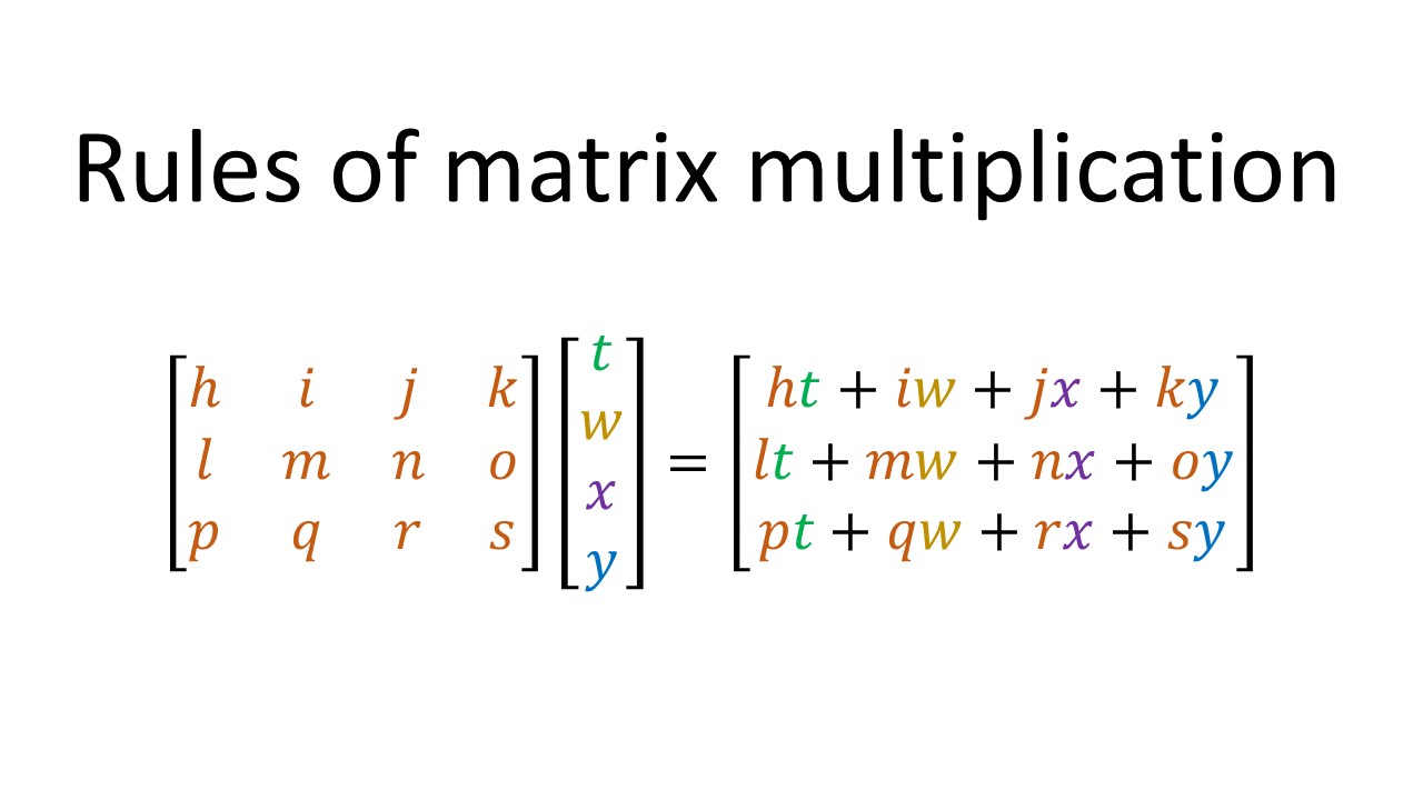
Matrix multiplication applied to our example:

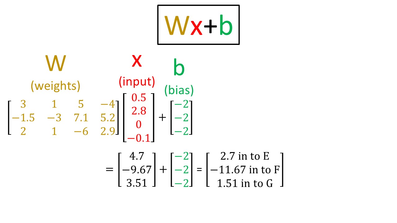
Here, I have taken all of the first-layer weights and arranged them in the gold matrix labeled W. I have taken the inputs x and arranged them as the red vector. The bias units are shown in green, and are all the same for a given layer (in this case they are all -2).

If you work through the matrix multiplication and bias addition, you see that we obtain exactly the same answer that we got before: 2.7 for node E, -11.67 for node F, and 1.51 for node G.

Recall that each of these numbers is subsequently squashed between 0 and 1 by the sigmoid function:

Obtaining the output

The final calculation for the output is shown here. Node E output value 0.937, node F output value 0.000009, and node G output value 0.819. Proceeding in the same way as before, we multiply each of these numbers by the corresponding weight (gold), sum them together, add the bias, and then apply the nonlinearity to get the final output of 0.388.

That is the “forward pass”: how neural networks compute an output prediction based on input data.

What about the backward pass?

Here, I will refer you to the excellent post by Matt Mazur, “A Step by Step Backpropagation Example.” If you work through his backpropagation example, I guarantee you will come away with a great understanding of how the backward pass works, i.e., how the neural network tweaks each of the weights to get a more correct answer the next time around.

The process of modifying the neural network to get a more correct answer is also referred to as “gradient descent.” The “gradient” is just the derivative of the loss function, and “descent” indicates that we are trying to go “down the derivative”, or make the loss function smaller. If you think of the loss function as a hill, we are trying to “descend” the hill so that our loss is smaller and our answer is less wrong (more correct).

Skiing down the loss function

The end! Stay tuned for future posts about multiclass vs. multilabel classification, different kinds of nonlinearities, and stochastic vs. batch vs. minibatch gradient descent!