

When training an image model, we want the model to be able to focus on important parts of the image. One way of accomplishing this is through trainable attention mechanisms. In this post we will first discuss the difference between post-hoc vs. trainable attention and soft vs. hard attention. We’ll then dive into the details of a 2018 ICLR paper, “Learn to Pay Attention” which describes one approach to trainable soft attention for image classification.
Key Paper Reference
Here is the key paper we will study in this post: Jetley S, Lord NA, Lee N, Torr PH. Learn to pay attention. ICLR 2018.
There is also a nice Pytorch implementation of the paper available here: SaoYan/LearnToPayAttention
Note: attention is also used extensively in natural language processing. The focus of this post is attention in computer vision tasks.
What is Attention?
Trainable vs. Post-Hoc Attention Mechanisms

Image Source
Let’s start with the English definition of the word “attention”:
attention: notice taken of someone or something; the regarding of someone or something as interesting or important
Similarly, in machine learning, “attention” refers to:
definition (1): trainable attention: a group of techniques that help a “model-in-training” notice important things more effectively
and
definition (2): post-hoc attention: a group of techniques that help humans visualize what an already-trained model thinks is important
When people think of attention, they usually think of definition (1), for trainable attention. A trainable attention mechanism is trained while the network is trained, and is supposed to help the network to focus on key elements of the image.
Confusingly, post-hoc heatmap visualization techniques are also sometimes referred to as “attention” which is why I’ve included definition (2). These post-hoc attention mechanisms create a heat map from an already-trained network, and include:
- heat maps via occlusion (Zeiler 2013)
- saliency maps (Simonyan 2013)
- CAM (Zhou 2016)
- Grad-CAM (Selvaraju 2017)
- HiResCAM (Draelos 2021), fixes a problem with Grad-CAM
I emphasize that these post-hoc techniques are not intended to change the way the model learns, or to change what the model learns. They are applied to an already-trained model with fixed weights, and are intended solely to provide insight into the model’s decisions.
Finally, let’s look at the definition of an “attention map” from Jetley et al:
attention map: a scalar matrix representing the relative importance of layer activations at different 2D spatial locations with respect to the target task
i.e., an attention map is a grid of numbers that indicates what 2D locations are important for a task. Important locations correspond to bigger numbers and are usually depicted in red in a heat map. In the following example, attention maps for “border collie” are shown, emphasizing the border collie’s position in the original montage:
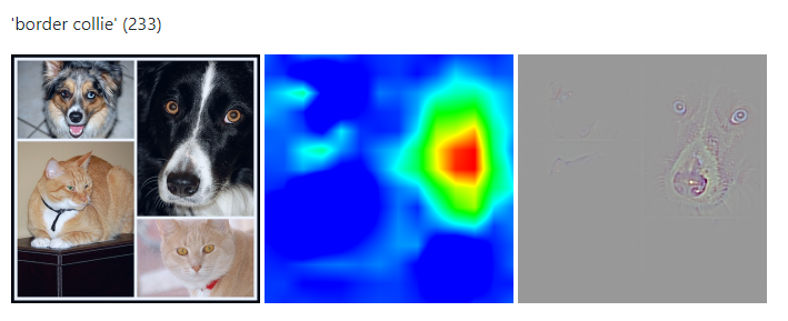
Image Source: ramprs/grad-cam
Soft vs. Hard Attention
You may have heard the terms “soft attention” and “hard attention” floating around. The difference between them is as follows:
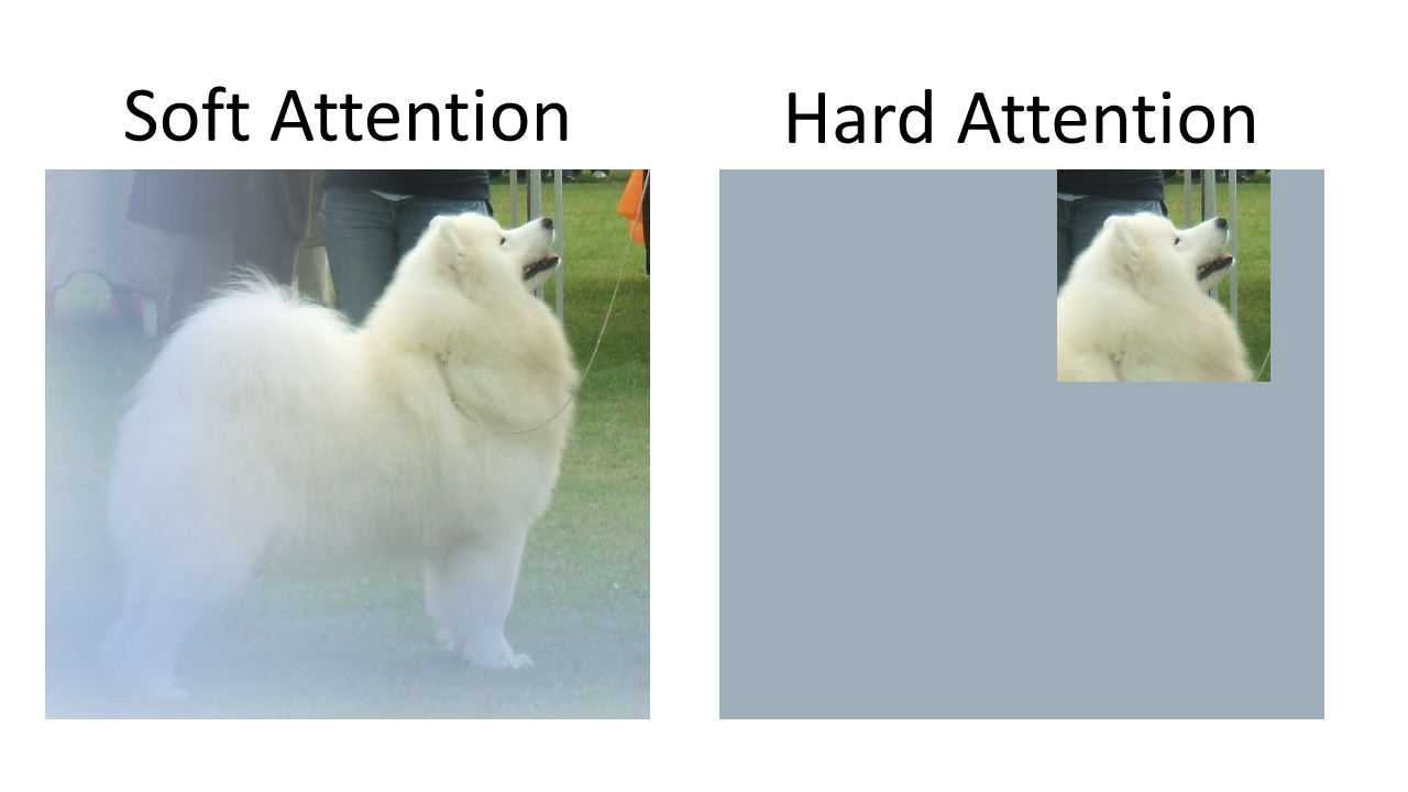
Modified from Image Source
- Soft attention uses “soft shading” to focus on regions. Soft attention can be learned using good old backpropagation/gradient descent (the same methods that are used to learn the weights of a neural network model.) Soft attention maps typically contain decimals between 0 and 1.
- Hard attention uses image cropping to focus on regions. It cannot be trained using gradient descent because there’s no derivative for the procedure “crop the image here.” Techniques like REINFORCE can be used to train hard attention mechanisms. Hard attention maps consistent entirely of 0 or 1, and nothing in-between; 1 corresponds to a pixel that is kept, and 0 corresponds to a pixel that is cropped out.
For more in-depth discussions of soft vs. hard attention, see this post (subsections “What is Attention?”, “Hard Attention,” and “Soft Attention”) and this post (subsection “Soft vs Hard Attention”).
Learn to Pay Attention
The paper “Learn to Pay Attention” demonstrates one approach to soft trainable visual attention in a CNN model. The main task they consider is multiclass classification, in which the goal is to assign an input image to a single output class, e.g. assign a photo of a bear to the class “bear.” The authors demonstrate that soft trainable attention improves performance on multiclass classification by 7% on CIFAR-100, and they show example heat maps highlighting how the attention helps the model focus on parts of the image most relevant to the correct class label.
Model Overview
Here’s a diagram of their model, modified from Figure 2 of the paper:
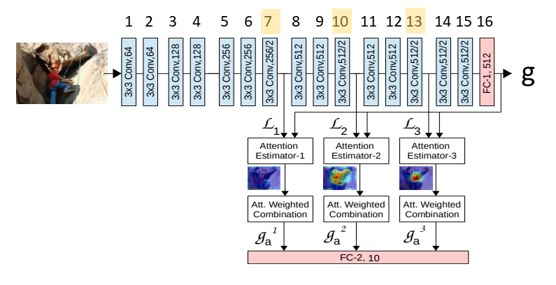
The model is based on the VGG convolutional neural network. There are different configurations of the VGG network, shown in Figure 2 here. (In case you’re curious, the “Learn to Pay Attention” paper appears to be using a VGG configuration somewhere between configurations D and E; specifically, there are three 256-channel layers like configuration D, but eight 512-channel layers like configuration E.)
The main point of this figure is that the authors have made two key changes to the basic VGG setup:
- They have inserted attention estimators after layers 7, 10, and 13 (the layer numbers that I’ve highlighted in yellow.) The attention estimator after layer 7 takes the output of layer 7 and calculates an “attention mask” of numbers between 0 and 1, which it then multiplies against the original output of layer 7 to produce “g_a^1” (in the figure above.) The same process happens for the attention estimators after layers 10 and 13, to produce g_a^2 and g_a^3, respectively.
- The next big change is that the authors have taken away the fully connected layer that normally goes at the end of VGG to produce the prediction (there’s normally another FC layer after the FC layer numbered “16” but they’ve gotten rid of it.) Instead, the classification now happens through a new fully connected layer that takes in inputs from the three attention estimators.
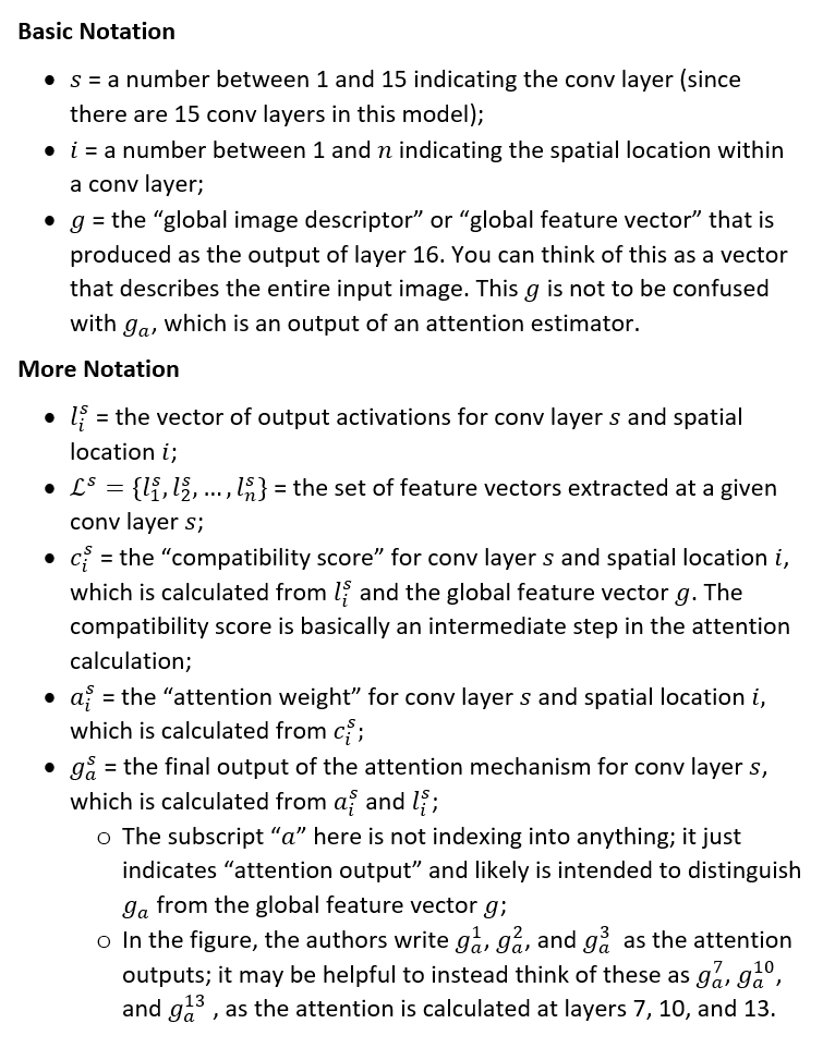
Notation
Before we dive into exactly how their attention mechanism works, here’s a summary of the notation used in the paper, which we will be using throughout the remainder of the post:
How the Attention Works
Step 1: Calculate the Compatibility Scores.
The “compatibility score” is calculated using the local features l and the global feature vector g.
The authors explain that the compatibility score is intended to have a high value when the image patch described by the local features “contains parts of the dominant image category.”
For example, if there’s a cat in the image, we assume that the whole cat is described by the global feature vector g, and furthermore, we expect that a particularly “cat-like” patch (e.g. a patch over the cat’s face) will produce local features l that produce a high compatibility score when combined with g.
The authors propose two different ways of calculating the compatibility score c from local features l and global feature vector g:
approach 1: “parametrised compatibiliy” or “pc”:
![]()
approach 2: “dot product” or “dp”:
![]()
(Spoiler alert: “parametrised compatibility” performed better in their results.)
In “parametrised compatibility” we first add the local features to the global feature, l+g, and then we take the dot product with a learned vector u. Intuitively it seems that concatenation of l and g might make more sense than addition, but the authors state, “given the existing free parameters between the local and the global image descriptors […] we can simplify the concatenation […] to an addition operation” in order to “limit the parameters of the attention unit.” (One of the reviewers also asked why they did addition instead of concatenation; see OpenReview.)
In the “dot product” approach we simply take the dot product of the local features l and the global feature vector g. Note that for each conv layer where we apply attention (layers 7, 10, and 13) the local features l will be unique to that layer but the global feature vector g is the same.
What if l and g are not the same size?
As it turns out, the l for conv layer 7 has 256 channels, but g has 512 channels. In order to add two vectors (pc approach) or take a dot product (dp approach), the vectors must be the same size.
The authors say that if l and g are not the same size, then they first project g to the lower-dimensional space of l. The reason they don’t instead project l to the higher-dimensional space of g is to limit the number of parameters. (By “project” they mean apply a neural network layer to make l the same size as g.)
Note that it’s still an acceptable solution to project l to g; you’ll just be making l bigger instead of making g smaller. This Pytorch implementation of “Learn to Pay Attention” projects l to g using the line “c1, g1 = self.attn1(self.projector(l1), g)” in which self.projector is a single convolutional layer that takes l which has an input of 256 channels and creates an output of 512 channels, to match g‘s 512 channels.
Step 2: Calculate the Attention Weights a from the Compatibility Scores c
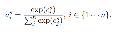
All we’re doing here is using a softmax to squish the compatibility scores c into the range (0,1) and we’re calling the output a. For a review of the softmax operation, see this post.
Step 3: Calculate the Final Output of the Attention Mechanism for Each Layer s.
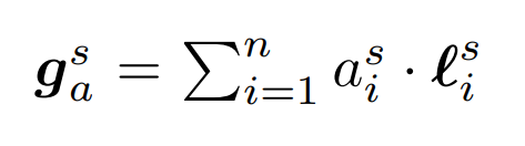
Here, we calculate the final output of the attention mechanism g_a for a particular layer s by taking a weighted combination of the l for that layer (recall that the l are just the outputs of that layer.) The weights we use are the attention weights a that we just calculated.
Step 4: Make a Classification Prediction Based on the Attention Final Output
Now we want to use the attention outputs g_a that we just calculated for layers 7, 10, and 13 to make a classification decision. The authors investigate two options:
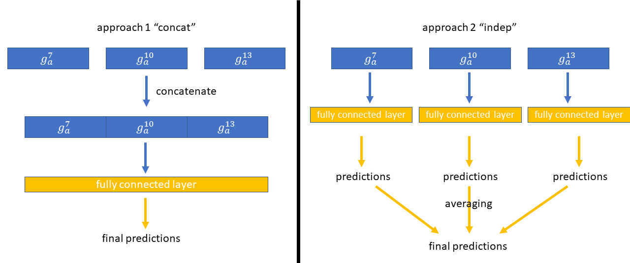
approach 1: “concat”: first concatenate the attention outputs and then feed them together into a single fully connected layer to get the final predictions.
approach 2: “indep”: feed each attention output into an independent fully connected layer to get intermediate predictions, then average those intermediate predictions to get the final predictions.
(Spoiler alert: “concat” performed better in their results.)
Results
Trainable Attention Improves Performance
The authors evaluate their attention mechanism on a variety of tasks, including multiclass classification with CIFAR-10, CIFAR-100, and SVHN. They find that use of their trainable attention mechanism improves performance over the “no-attention” baseline, in contrast to one of the post-hoc attention mechanisms (CAM) which results in a decrease in performance (due to the architecture constraints imposed by the CAM approach.)
The following variant of their method performed best: “parametrised compatibility” (calculating compatibility scores by adding l and g and then taking the dot product with a learned vector u) and “concat” (concatenating the attention outputs g_a before feeding them into an fc layer to make predictions.)
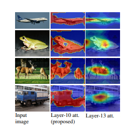
Here’s part of Figure 3 from their paper showing some example attention maps focused on relevant objects:
How useful is the global feature vector g?
The appendix of their paper contains an interesting discussion on the utility of the global feature vector g in the calculation of the attention. Recall that both the “pc” and “dp” approaches for obtaining compatibility scores make use of the global feature vector g. The authors ran experiments where they swapped out which g they used, and found:
- for the dot-product-based attention mechanism [dp, worse-performing]: “the global vector plays a prominent role in guiding attention”
- for the parametrised compatibility function [pc, better-performing]: “the global feature vector seems to be redundant. Any change in the global feature vector does not transfer to the resulting attention map. In fact, numerical observations show that the magnitudes of the global features are often a couple orders of magnitude smaller than those of the corresponding local features. Thus, a change in the global feature vector has little to no impact on the predicted attention scores. Yet, the attention maps themselves are able to consistently highlight object-relevant image regions. Thus, it appears that in the case of parametrised compatibility based attention, the object-centric high-order features are learned as part of the weight vector u.”
In other words, we might be able to get away with calculating the compatibility scores like this:
![]()
without using g at all!
Regardless of the exact role that g is playing, this “Learn to Pay Attention” method does improve results, and does produce nice attention maps – so the trainable attention is clearly doing something useful, even if it’s not using g in the exact way the authors initially intended.
Summary
- Trainable attention mechanisms have attention weights that are learned during training, which help the model focus on key parts of images important for the task;
- Post-hoc attention mechanisms are techniques applied after a model is finished training, and are intended to provide insight into where the model is looking when it makes predictions;
- Hard attention is image cropping and can be trained using REINFORCE. Soft attention produces “hazier” focus region(s) and can be trained using regular backpropagation.
- “Learn to Pay Attention” is an interesting paper demonstrating how soft trainable attention can improve image classification performance and highlight key parts of images.
Additional Resources
- Attention in Neural Networks and How to Use It by Adam Kosiorek. This is a great article focused on attention in computer vision. It discusses why attention is useful, soft vs hard attention, Gaussian attention (with code), and Spatial Transformers (with code).
- Attention? Attention! by Lilian Weng. This is another great article, focused on attention in natural language processing. It discusses seq2seq, self-attention, soft vs. hard attention, global vs. local attention, Neural Turing Machines, Pointer Networks, Transformers, SNAIL, and Self-Attention GAN.
- The Transformer: Attention Is All You Need: explains the Transformer, including its multi-head trainable self-attention mechanism.
- CNN Heat Maps: Saliency/Backpropagation: explains the post-hoc attention technique saliency mapping.
- CNN Heat Maps: Gradients vs. DeconvNets vs. Guided Backpropagation: explains how these three post-hoc attention methods are actually identical to each other, except for handling of nonlinearities.
- CNN Heat Maps: Class Activation Mapping (CAM): explains the class activation mapping architecture and attention mechanism, which along with HiResCAM is provably guaranteed to show where a model is looking.
- Guided Grad-CAM is Broken! Sanity Checks for Saliency Maps: explains a NeurIPS paper that reveals problems with several popular attention mechanisms.
- Grad-CAM: Visual Explanations from Deep Networks: explains the post-hoc attention mechanism Grad-CAM. Note: although the Grad-CAM paper has been cited several thousand times, recent work demonstrates a serious issue with Grad-CAM, namely that it sometimes highlights irrelevant regions the model did not actually use.
About the Featured Image
Image Source: Performer with fire poi. Poi is a performing art focused on swinging tethered weights. It originated in New Zealand.
Want to be the first to hear about my articles bridging healthcare, artificial intelligence, and business—and get a free list of my favorite health AI resources? Sign up here.

#/media/File:Flammenjongleur.jpg)
Comments are closed.