The Transformer: Attention Is All You Need

The Transformer paper, “Attention is All You Need” is the #1 all-time paper on Arxiv Sanity Preserver as of this writing (Aug 14, 2019). This paper showed that using attention mechanisms alone, it’s possible to achieve state-of-the-art results on language translation. Subsequent models built on the Transformer (e.g. BERT) have achieved excellent performance on a wide range of natural language processing tasks.

Throughout this post, I use a mixture of custom figures, figures modified from the original paper, equations, tables, and code, in an effort to explain the Transformer as clearly as possible. By the end of this post, you should understand all the different pieces of the Transformer model:

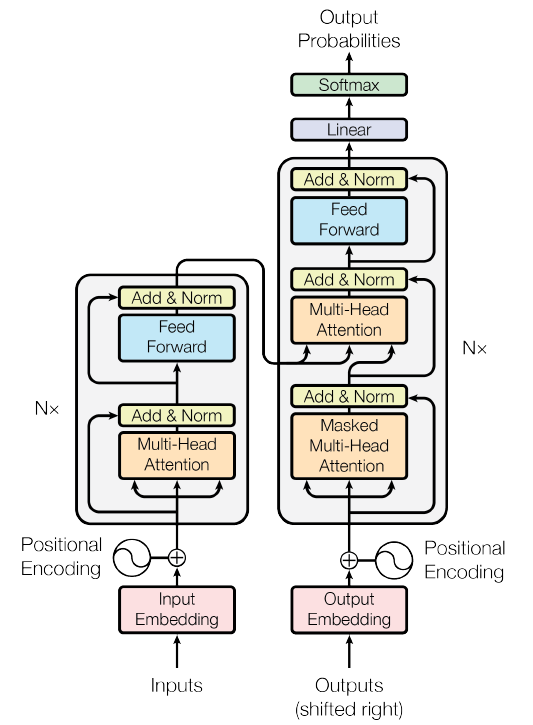
Figure 1 from the Transformer paper

Paper

Vaswani A, Shazeer N, Parmar N, Uszkoreit J, Jones L, Gomez AN, Kaiser Ł, Polosukhin I. Attention is all you need. NeurIPS 2017 (pp. 5998-6008).

All quotes in this post are from the paper.

Code

For a Pytorch implementation of the Transformer model, please see “The Annotated Transformer” which is an iPython notebook containing the Transformer paper text interspersed with working Pytorch code. I will reference code from the Annotated Transformer throughout this post, and explain certain sections of the code in detail.

Note that the order in which we will discuss parts of the Transformer here is different from the order in either the original paper or the Annotated Transformer. Here, I’ve organized everything according to the flow of data through the model, e.g. starting from an English sentence “I like trees” and working through the Transformer to a Spanish translation “Me gustan los arboles.”

The hyperparameters used here are those of the Transformer base model, as shown in this excerpt from Table 3 of the Transformer paper:

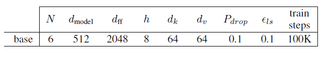
These are the same hyperparameters used in the code in the function “make_model(src_vocab, tgt_vocab, N=6, d_model=512, d_ff = 2048, h=8, dropout=0.1).”

Representing Inputs and Outputs

For English-Spanish language translation, the input to the Transformer is an English sentence (“I like trees”) and the output is the Spanish translation of that sentence (“Me gustan los arboles”).

Representing the Input

We first represent each word of the input sentence using a one-hot vector. A one-hot vector is a vector in which every element is “zero,” except for a single element which is a “one”:

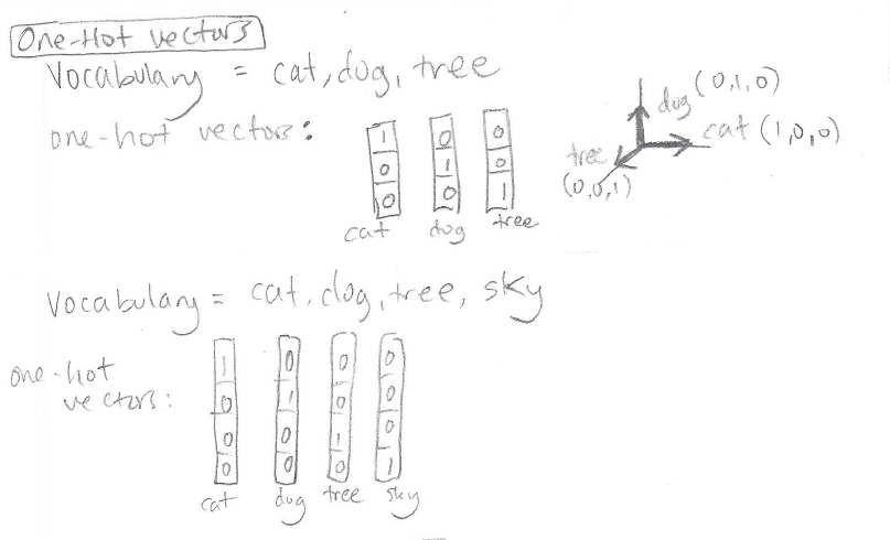
The length of each one-hot vector is determined beforehand by the size of the vocabulary. If we want to represent 10,000 different words we need to use one-hot vectors of length 10,000 (so that we have a unique slot for the “one” for each word.) For more background on one-hot vectors, please see the post Preparing Tabular Data for Neural Networks (Code Included!), Section “Representing Categorical Variables: One-Hot Vectors.”

Word Embeddings

We don’t want to feed the Transformer plain one-hot vectors because they’re sparse, huge, and tell us nothing about the characteristics of the word. Therefore we learn a “word embedding” which is a smaller real-valued vector representation of the word that carries some information about the word. We can do this using nn.Embedding in Pytorch, or, more generally speaking, by multiplying our one-hot vector with a learned weight matrix W.

nn.Embedding consists of a weight matrix W that will transform a one-hot vector into a real-valued vector. The weight matrix has shape (num_embeddings, embedding_dim). num_embeddings is simply the vocabulary size – you need one embedding for each word in the vocabulary. embedding_dim is the size you want your real-valued representation to be; you can choose this to be whatever you want – 3, 64, 256, 512, etc. In the Transformers paper they choose 512 (the hyperparameter d_model = 512).

People refer to nn.Embedding as a “lookup table” because you can imagine the weight matrix as merely a stack of the real-valued vector representations of the words:

There are two options for dealing with the Pytorch nn.Embedding weight matrix. One option is to initialize it with pre-trained embeddings and keep it fixed, in which case it’s really just a lookup table. Another option is to initialize it randomly, or with pre-trained embeddings, but keep it trainable. In that case the word representations will get refined and modified throughout training because the weight matrix will get refined and modified throughout training.

The Transformer uses a random initialization of the weight matrix and refines these weights during training – i.e. it learns its own word embeddings.

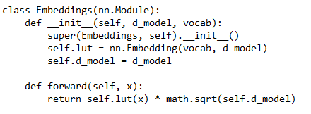
In the Annotated Transformer the word embeddings are created using the class “Embeddings” which in turn makes use of nn.Embedding:

Positional Encoding

We could just feed in the word embeddings for each word in our sentence and use that as our input representation. However, the word embeddings alone don’t carry any information about the relative order of words in the sentence:

• “I like trees” and “The trees grew” both contain the word “trees”
• The word “trees” has the exact same word embedding regardless of whether it’s the third word or second word in a sentence.

In an RNN, it would okay to use the same vector for the word “trees” everywhere, because the RNN processes an input sentence sequentially, one word at a time. However, in a Transformer, all words in the input sentence are processed simultaneously – there is no inherent “word ordering” and thus no inherent position information.

The authors of the Transformer propose adding a “positional encoding” to address this problem. The positional encoding makes it possible for the Transformer to use information about word order. The positional encoding uses a sequence of real-valued vectors that capture ordering information. Each word in a sentence is summed with a particular positional encoding vector based on its position within the sentence:

How exactly does the “position vector” carry information about position? The authors explored two options for creating the positional encoding vectors:

• option 1: learning the positional encoding vectors (requires trainable parameters),
• option 2: calculating the positional encoding vectors using an equation (requires no trainable parameters)

They found the performance of both options was similar, so they went with the latter option (calculation) because it requires no parameters and also might allow the model to work well even on sentence lengths not seen during training.

Here’s the formula they use to calculate the positional encoding:

In this equation,

• pos is the position of a word in the sentence (e.g. “2” for the second word in the sentence)
• i indexes into the embedding dimension, i.e. it’s the position along the positional encoding vector dimension. For a positional encoding vector of length d_model = 512, we’ll have i range from 1 to 512.

Why use sine and cosine? To quote the authors, “each dimension of the positional encoding corresponds to a sinusoid. […] We chose this function because we hypothesized it would allow the model to easily learn to attend by relative positions.”

In the Annotated Transformer the positional encoding is created and added to the word embeddings using the class “PositionalEncoding”:

Summary of the Input

Now we’ve got our input representation: an English sentence, “I like trees” converted to three vectors (one vector for each word):

Each of the vectors in our input representation captures both the word’s meaning and the word’s position in the sentence.

We’ll do the exact same process (word embedding + positional encoding) to represent the output, which in this case is the Spanish sentence “Me gustan los arboles.”

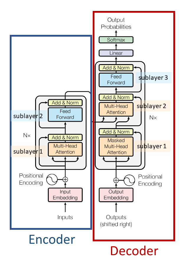
Now we’ve covered the bottom piece of Figure 1 of the Transformers paper: how the input and output sentences are processed before being fed into the rest of the model (not to be confused with the “output probabilities” at the top, which are something else):

The shape of the inputs Tensor (and of the outputs Tensor) after the embedding and positional encoding is [nbatches, L, 512] where “nbatches” is the batch size (to follow the Annotated Transformer’s variable name), L is the length of the sequence (e.g. L = 3 for “I like trees”), and 512 is the embedding dimension / positional encoding dimension. Note that the batches are created carefully such that a single batch contains sequences of similar length.

The Encoder

Now it’s time for the encoder to process our sentence. Here’s what the encoder looks like:

Figure modified from Transformer paper Figure 1.

As you can see from the figure, the encoder is made of N = 6 identical layers stacked on top of each other.

For English-Spanish translation, what goes “in” is an English sentence, e.g. “I like trees,” represented in the “word embeddings + positional encodings” format we just talked about. What comes “out” is a different representation of this sentence.

Each of the six encoder layers contains two sub-layers:

• the first sub-layer is “a multi-head self-attention mechanism”
• the second sub-layer is “a simple, position-wise fully connected feed-forward network”

Figure modified from Transformer paper Figure 1.

We’ll talk about what each of these sub-layers is doing. But first, here’s code from the Annotated Transformer showing how the Encoder is built:

• The class “Encoder” takes in a <layer> and stacks it <N> times. The <layer> that it takes in is an instance of the class “EncoderLayer”
• The class “EncoderLayer” is initialized with <size>, <self_attn>, <feed_forward>, and <dropout>:
  • <size> is d_model, which is 512 in the base model
  • <self_attn> is an instance of class “MultiHeadedAttention.” This corresponds to sub-layer 1.
  • <feed_forward> is an instance of class “PositionwiseFeedForward.” This corresponds to sub-layer 2.
  • <dropout> is the dropout rate, e.g. 0.1

Encoder Sub-Layer 1: Multi-Head Attention Mechanism

Cerberus the multi-headed dog (Image Source)

It is critical to understand the multi-head attention mechanism in order to understand the Transformer. The multi-head attention mechanism is used in both the encoder and the decoder. First I’ll write a high-level summary based on the equations from the paper, and then we’ll dive into the details of the code.

High-Level Verbal Summary of Attention: Keys, Queries, and Values

Let’s call our input to the attention mechanism “x.” At the beginning of the encoder, x is our initial sentence representation. In the middle of the encoder, “x” is the output of the previous EncoderLayer. For example EncoderLayer3 gets its input “x” from the output of EncoderLayer2.

We use x to calculate keys, queries, and values. The keys, queries, and values are calculated from x using distinct linear layers:

• key = linear_k(x)
• query = linear_q(x)
• value = linear_v(x)

where for a particular encoder layer, linear_k, linear_q, and linear_v are separate feedforward neural network layers that go from dimension 512 to dimension 512 (d_model to d_model.) Linear_k, linear_q, and linear_v have different weights from each other which are learned separately. If we used the same layer weights to calculate the keys, queries, and values, then they’d all be identical to each other and we wouldn’t need different names for them.

Once we have our keys (K), queries (Q), and values (V), we calculate the attention as follows:

This is equation (1) in the Transformer paper. Let’s dissect what is going on:

First, we take the dot product between the query and the key. If we do this on many queries and keys simultaneously, we can write the dot products as a matrix multiplication like so:

Here Q is a stack of queries q, and K is a stack of keys k.

After we take the dot product, we divide by the square root of d_k:

What’s the point of dividing by sqrt(d_k)? The authors explain that they scale the dot products by sqrt(d_k) to prevent the dot products from getting huge as d_k (the vector length) increases.

Example: the dot product of the vectors [2,2] and [2,2] is 8, but the dot product of the vectors [2,2,2,2,2] and [2,2,2,2,2] is 20. We don’t want the dot product to be huge if we choose a huge vector length, so we divide by the square root of the vector length to mitigate this effect. A huge dot product value is bad because it will “push the softmax function into regions where it has extremely small gradients.”

Which brings us to the next step – applying a softmax, which squishes the numbers into a (0,1) range:

For a discussion of the softmax function see this post.

What do we have at this point? At this point, we have a bunch of numbers between 0 and 1, which we can think of as our attention weights. We’ve calculated these attention weights as softmax(QK^T/sqrt(d_k)).

The last step is to do a weighted sum of the values V, using the attention weights that we just calculated:

And that’s the whole equation!

More Detailed Description of Multi-Headed Attention with Code

This section refers to code from the Annotated Transformer, as I think looking at the code is a good way to understand what is happening.

First, here are the relevant pieces of code with some annotations. Don’t worry about all these annotations – I’ll describe the key points in the text below. (If you would like to read the annotations, depending on your browser you may have to open the image in a new window in order for the text to be large enough to read.)

In the Annotated Transformer, multi-headed attention is implemented with the class MultiHeadedAttention:

An instance of this class is initialized with:

• <h> = 8, the number of “heads.” There are 8 heads in the Transformer base model.
• <d_model> = 512
• <dropout> = dropout rate = 0.1

The dimension of the keys, d_k, is calculated as d_model/h. So in this case, d_k = 512/8 = 64.

Let’s look in more detail at the forward() function from MultiHeadedAttention:

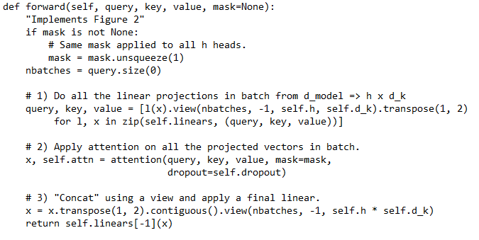
We can see that the input to forward() is query, key, value, and mask. Ignore the mask for now. Where do the query, key, and value come from? They are in fact from the “x” repeated three times in the EncoderLayer (see yellow highlight):

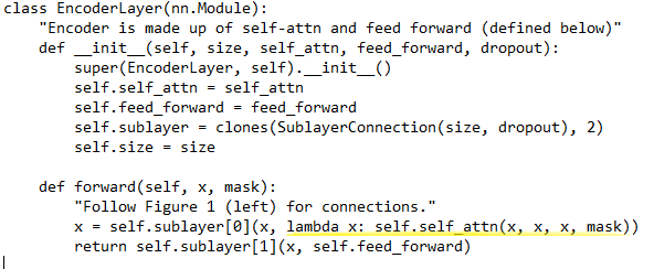
The x came from the previous EncoderLayer, or if we’re at EncoderLayer1, the x is our initial sentence representation. (Note that self.self_attn in class EncoderLayer is an instance of MultiHeadedAttention.)

Within the MultiHeadedAttention class, we’re going to take the old queries (the old x), the old keys (also the old x), and the old values (also the old x), and produce new queries, keys, and values which are distinct from each other.

Note that the shape of the “query” input is [nbatches, L, 512] where nbatches is the batch size, L is the sequence length, and 512 is d_model. The “key” and “value” inputs also have shape [nbatches, L, 512].

Step 1) in the MultiHeadedAttention forward() function states, “Do all the linear projections in batch from d_model => h x d_k.”

• We’ll do three different linear projections on the same Tensor of shape [nbatches, L, 512] to obtain new queries, keys, and values, each of shape [nbatches, L, 512]. (The shape hasn’t changed since the linear layer is 512 –> 512).
• Then, we’ll reshape that output into 8 different heads. For example the queries are shape [nbatches, L, 512] and are reshaped using view() to [nbatches, L, 8, 64] where h=8 is the number of heads and d_k = 64 is the key size.
• Finally we’ll swap dimensions 1 and 2 using transpose to get shape [nbatches, 8, L, 64]

Step 2) in the code states, “Apply attention on all the projected vectors in batch.”

• The specific line is x, self.attn = attention(query, key, value, mask=mask, dropout=self.dropout)
• Here’s the equation we’re implementing using the attention() function:

• And here’s the attention() implementation:

To calculate the scores, we first do a matrix multiplication between query [nbatches, 8, L, 64] and key transposed [nbatches, 8, 64, L]. This is the QK^T from the equation. The resulting shape of scores is [nbatches, 8, L, L].

Next, we calculate the attention weights p_attn by applying a softmax to the scores. If applicable, we also apply dropout to the attention weights. p_attn thus corresponds to softmax(QK^T/sqrt(d_k)) in the equation above. The shape of p_attn is [nbatches, 8, L, L] because applying softmax and dropout to the scores doesn’t change the shape.

Finally, we perform a matrix multiplication between the attention weights p_attn [nbatches, 8, L, L] and the values [nbatches, 8, L, 64]. The result is the final output of our attention function, with shape [nbatches, 8, L, 64]. We return this from the function, along with the attention weights themselves p_attn.

Notice that in our input to the attention function and in the output of the attention function, we have 8 heads (dimension 1 of our Tensor, e.g. [nbatches, 8, L, 64].) We did a different matrix multiplication for each of the eight heads. This is what is meant by “multi-headed” attention: the extra “heads” dimension allows us to have multiple “representation subspaces.” It gives us eight different ways of considering the same sentence.

Step 3) (in the MultiHeadedAttention class, since we’ve now returned from the attention() funtion) is concatenation using a view() followed by application of a final linear layer.

• The specific lines of Step 3 are:

    x = x.transpose(1, 2).contiguous().view(nbatches, -1, self.h * self.d_k)

        return self.linears[-1](x)

• x is what’s returned from the attention function: our eight-headed representation [nbatches, 8, L, 64].
• We transpose it to get [nbatches, L, 8, 64] and then reshape it using view to get [nbatches, L, 8 x 64] = [nbatches, L, 512]. This reshaping operation using view() is basically a concatenation across the 8 heads.
• Finally, we apply our last linear layer from self.linears. This linear layer goes from 512 –> 512. Note that in Pytorch if a multi-dimensional Tensor is given to a Linear layer, the Linear layer is applied only to the last dimension. So the result of self.linears[-1](x) still has shape [nbatches, L, 512].
• Notice that [nbatches, L, 512] is exactly the right shape we need to feed in to another MultiHeadedAttention layer….
• …But before we do that, we’ve got one last step, Encoder Sub-Layer 2, which we’ll talk about right after we review Figure 2 from the Transformer paper.

Here is Figure 2 from the Transformer paper:

Transformer paper Figure 2

On the left, under “Scaled Dot-Product Attention” we have a visual depiction of what the attention() function calculates: softmax(QK^T/sqrt(d_k))V. It’s “scaled” because of the division by sqrt(d_k) and it’s “dot-product” because QK^T represents the dot product between a bunch of stacked queries and a bunch of stacked keys.

On the right, under “Multi-Head Attention” we have a visual depiction of what the MultiHeadedAttention class does. You should now recognize the parts of this figure:

• At the bottom going in are the old V, K, and Q, which are our “x” output from a previous EncoderLayer (or our x from the input sentence representation for EncoderLayer1)
• Next we apply a Linear layer (the “Linear” boxes) to calculate a processed V, K, and Q (which are not explicitly shown)
• We feed the processed V, K, and Q into our scaled dot-product attention with 8 heads. This is the attention() function.
• Finally, we concatenate the result of the attention() function over the 8 heads, and apply a last linear layer to produce our multi-headed attention output.

Encoder Sub-Layer 2: Position-Wise Fully Connected Feed-Forward Network

We are now almost done understanding an entire EncoderLayer! Recall that this is the basic structure of a single EncoderLayer (modified from Transformer paper Figure 1):

We’ve gone over sub-layer 1, the multi-head attention. Now we’ll take a look at sub-layer 2, the feed-forward network.

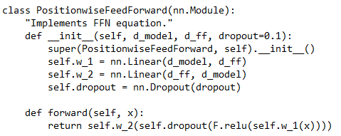
Sub-layer 2 is easier to understand than sub-layer 1, because sub-layer 2 is just a feedforward neural network. Here’s the expression for sub-layer 2:

In other words, we apply a fully-connected layer with weights W1 and biases b1, perform a ReLU nonlinearity (the max with zero), and then apply a second fully-connected layer with weights W2 and biases b2.

Here’s the corresponding code snippet from the Annotated Transformer:

So, in summary, the Encoder consists of 6 EncoderLayers. Each EncoderLayer has 2 sub-layers: sub-layer 1 for multi-headed attention, and sub-layer 2 that’s just a feedforward neural network.

The Decoder

Now that we understand the encoder, the decoder will be easier to understand, because it’s similar to the encoder. Here’s Figure 1 again, with a few extra annotations:

Modified from Transformer paper Figure 1

Here are three main differences between the decoder and the encoder:

• Decoder sub-layer 1 uses “masked” multi-head attention to prevent illegally “seeing into the future.”
• The decoder has an extra sub-layer, labeled “sub-layer 2” in the figure above. This sub-layer is “encoder-decoder multi-head attention.”
• There is a linear layer and a softmax applied to the decoder output to produce output probabilities which indicate the next predicted word.

Let’s talk about each of these pieces.

Decoder Sub-Layer 1: Masked Multi-Head Attention

The Crystal Ball by John William Waterhouse

The point of masking in the multi-headed attention layer is to prevent the decoder from “seeing into the future”  – i.e. we don’t want any crystal balls built into our model.

The mask consists of ones and zeros:

Mask example (Image Source).

The lines of code in the attention() function that use the mask are here:

    if mask is not None:

        scores = scores.masked_fill(mask == 0, -1e9)

The masked_fill(mask, value) function “fills elements of self tensor with value where mask is True. The shape of mask must be broadcastable with the shape of the underlying tensor.” So, basically, we use the mask to “zero out” parts of the scores Tensor that correspond to future words we aren’t supposed to see.

To quote the authors, “We […] modify the self-attention sub-layer in the decoder stack to prevent positions from attending to subsequent positions. This masking, combined with fact that the output embeddings are offset by one position, ensures that the predictions for position i can depend only on the known outputs at positions less than i.”

Decoder Sub-Layer 2: Encoder-Decoder Multi-Head Attention

Here’s the code for a DecoderLayer:

The line underlined in yellow defines the “encoder-decoder attention”:

        x = self.sublayer[1](x, lambda x: self.src_attn(x, m, m, src_mask))

self.src_attn is an instance of MultiHeadedAttention. The inputs are query = x, key = m, value = m, and mask = src_mask. Here, x comes from the previous DecoderLayer, while m or “memory” comes from the output of the Encoder (i.e. the output of EncoderLayer6).

(Note that the line above the line in yellow, x = self.sublayer[0](x, lambda x: self.self_attn(x, x, x, tgt_mask)), defines the decoder self-attention of decoder sub-layer 1 that we just talked about. It works exactly the same way as encoder self-attention except for the extra masking step.)

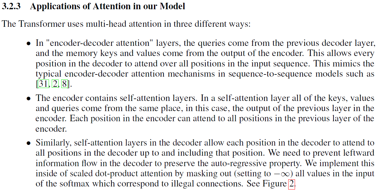
Aside: Complete Summary of Attention in the Transformer

We’ve now gone over the three kinds of attention in the Transformer. Here’s the author summary from the Transformer paper about the three ways attention is used in their model:

Decoder Final Output: Linear and Softmax to Produce Output Probabilities

At the end of the decoder stack, we feed the decoder’s final output into a linear layer followed by a softmax, to predict the next token.

We ran the encoder once to get the output of the encoder stack, which represents the English input sentence “I like trees”; now we’re going to run the decoder multiple times so it can predict the multiple words in the Spanish translation “Me gustan los arboles.”

The last linear layer expands the output of the decoder stack into a huge vector whose length is equal to the vocabulary size. The softmax means that we’ll select the one element of this huge vector with the highest probability (“greedy decoding”) which corresponds to one word in our Spanish vocabulary.

After the network is trained (i.e. when we’re performing inference), we’ll do the following steps (note that the encoder output is calculated once and then used several times):

1. Feed the decoder our encoder output (which represents the full English sentence “I like trees”) and a special beginning of sentence token, </s>, in the “output sentence” slot at the bottom of the decoder. The decoder will produce a predicted word, which in our example should be “Me” (the first word of our Spanish translation.) 
2. Feed the decoder our encoder output, the beginning of sentence token, and the word the decoder just produced – i.e., feed the decoder the encoder output and “</s> Me.” In this step the decoder should produce the predicted word “gustan.”
3. Feed the decoder our encoder output and “</s> Me gustan.” In this step the decoder should produce the predicted word “los.”
4. Feed the decoder our encoder output and “</s> Me gustan los.” In this step the decoder should produce the predicted word “arboles.”
5. Feed the decoder our encoder output and “</s> Me gustan los arboles.” In this step the decoder should produce the end-of-sentence token , for example “</eos>.”
6. Because the decoder has produced an end-of-sentence token, we know we are done translating this sentence.

What about during training? During training, the decoder might not be very good – so it can produce incorrect predictions of the next word. If the decoder is producing junk, we don’t want to feed that junk back into the decoder for the next step. So, during training we use a process called “teacher forcing” (ref1, ref2, ref3).

In teacher forcing, we make use of the fact that we know what the correct translation should be, and we feed the decoder the symbols that it should have predicted so far. Note that we don’t want the decoder to just learn a copying task, so we’ll only feed it “</s> Me gustan los” at the step where it’s supposed to be predicting the word “arboles.” This is implemented through:

• the masking that we talked about earlier, in which future words are zeroed out (i.e. no feeding the decoder “los arboles” when it’s supposed to be predicting “gustan”), and
• a right-shift so that the “present” word isn’t fed in either (i.e. no feeding the decoder “gustan” when it’s supposed to be predicting “gustan.”)

The loss is then calculated using the probability distribution over possible next words that the decoder actually produced (e.g. [0.01,0.01,0.02,0.7,0.20,0.01,0.05]), versus the probability distribution it should’ve produced (which is [0,0,0,0,1,0,0] with the “1” in the “arboles” slot if we’re using one-hot vectors as ground truth.)

Note that the approach I just described (selecting the highest-probability word at each decoding step) is called “greedy decoding.” An alternative is beam search, which keeps more than one predicted word at each decoding step (see this post for more details.)

Here’s the Pytorch Generator class used for the final linear layer and softmax:

More Fun

Congratulations – you have just worked through the key parts of a Transformer model! There are a few additional concepts built in to the Transformer that I’ll overview quickly here:

Dropout: dropout is used in a few different places throughout the Transformer. In this technique, a random subset of neurons are ignored during each forward/backward pass to help prevent overfitting. For more information on dropout see this post.

Residual Connection and Layer Normalization: There’s a residual connection around each sub-layer of the encoder and around each sub-layer of the decoder, followed by layer normalization.

• Residual connection: if we calculate some function f(x), a “residual connection” produces the output f(x)+x. In other words, we add the original input back onto the output that we just calculated. For more details see this article.
• Layer normalization: this is a method that normalizes inputs across the features (as opposed to batch normalization which normalizes features across a batch.) For more details see this article.

In the following diagram of an EncoderLayer I’ve colored red the relevant parts: the arrow and the “Add and Norm” box that together represent the residual connection and the layer normalization:

Modified from Transformer paper Figure 1.

Quote, “the output of each sub-layer is LayerNorm(x + Sublayer(x)), where Sublayer(x) is the function implemented by the sub-layer itself. To facilitate these residual connections, all sub-layers in the model, as well as the embedding layers, produce outputs of dimension dmodel = 512.”

For the Pytorch implementation, see the Annotated Transformer class “LayerNorm” as well as class “SublayerConnection” which applies LayerNorm, Dropout, and a residual connection.

Noam optimizer: The Transformer is trained using the Adam optimizer. The authors report a specific formula for varying the learning rate throughout training. First the learning rate is increased linearly for a certain number of training steps. After that, the learning rate is decreased proportionally to the inverse square root of the step number. This learning rate schedule is implemented in the Annotated Transformer class “NoamOpt.”

Label smoothing: Finally, the authors apply the label smoothing technique. Essentially, label smoothing takes one-hot-encoded “correct answers” and smooths them out so that most of the probability mass goes where the “1” was, and the remainder is distributed throughout all the slots that were “0.” For more details see this paper. For the implementation see Annotated Transformer class “LabelSmoothing.”

Grand Summary!

• The Transformer consists of an Encoder and a Decoder.
• The input sentence (e.g. “I like trees”) and the output sentence (e.g. “Me gustan los arboles”) are each represented using a word embedding plus positional encoding vector for each word.
• The Encoder is made up of 6 EncoderLayers. The Decoder is made up of 6 DecoderLayers.
• Each EncoderLayer has two sub-layers: multi-headed self-attention and a feedforward layer.
• Each DecoderLayer has three sub-layers: multi-headed self-attention, multi-headed encoder-decoder attention, and a feedforward layer.
• At the end of the Decoder, a linear layer and a softmax are applied to the Decoder output to predict the next word.
• The Encoder is run once. The Decoder is run multiple times, to produce a predicted word at each step.

References

• Vaswani A, Shazeer N, Parmar N, Uszkoreit J, Jones L, Gomez AN, Kaiser Ł, Polosukhin I. “Attention is all you need.” NeurIPS 2017 (pp. 5998-6008).
• The Annotated Transformer by Harvard NLP. An iPython notebook that walks through the paper step-by-step with working Pytorch code throughout.
• Walkthrough: The Transformer Architecture [Part 1/2] by Matthew Barnett. Overview of basic concepts in the Transformer without excess details.
• Walkthrough: The Transformer Architecture [Part 2/2] by Matthew Barnett. Details about how the Transformer works. Great post for explaining what queries, keys, and values actually are.
• The Illustrated Transformer by Jay Alammar
• Transformer Tutorial – DGL 0.3 documentation. Includes an interesting graph illustration of the decoder/encoder
• CS224N Transformer Networks by Richard Socher
• Transformer model for language understanding from Tensorflow Core. Includes Tensorflow example code.

About the Featured Image

The featured image is a crop from the painting “The Crystal Ball” by John William Waterhouse.