

Certain techniques for understanding what a CNN is looking at don’t work. They have no connection to the model’s weights or to the training data, and may be merely acting as edge detectors.
In this post we will discuss the NeurIPS 2018 paper, “Sanity Checks for Saliency Maps” which demonstrates that several popular saliency map approaches do not in fact provide insight into what a model is doing. Models with randomized weights and models trained on data with randomized labels will still produce convincing-looking “explanations” for certain saliency map techniques, including Guided GradCAM and Guided Backpropagation, which means that these saliency map approaches aren’t related to the model’s parameters or the training data.
Paper
The following paper applies several clever sanity checks to determine whether a particular technique provides insight into a model or not:
Any quotes in this post are from this paper unless otherwise noted.
CNN Saliency Map (Heat Map) Techniques
Here are the saliency map techniques that this paper evaluates:
- Gradient: In this technique, we visualize how much a change in each of the input pixels changes the final predictions. The Gradient is the derivative of the score with respect to the input image, and is sometimes referred to as “Saliency” or “Backpropagation.” For more details, see CNN Heat Maps: Saliency/Backpropagation and CNN Heat Maps: Gradients vs. DeconvNets vs. Guided Backpropagation.
- SmoothGrad (SG): This is a technique for smoothing out saliency maps by taking an average over the saliency maps produced from noisy copies of an input.
- Gradient x Input: This is the element-wise product of the input and the gradient.
- Integrated Gradients (IG): This gradient-based technique sums over scaled versions of the input.
- Guided Backpropagation (GBP): This approach differs from the gradients approach only at the ReLU nonlinearity. For a detailed explanation, see CNN Heat Maps: Gradients vs. DeconvNets vs. Guided Backpropagation.
- GradCAM: “GradCAM explanations correspond to the gradient of the class score (logit) with respect to the feature map of the last convolutional unit.” GradCAM is built off of CAM. For details on CAM see CNN Heat Maps: Class Activation Mapping.
- Guided GradCAM: This is an element-wise product of GradCAM with Guided Backpropagation.
Passing or Failing the Sanity Checks
The short summary from the authors: “Of the methods we tested, Gradients and GradCAM pass the sanity checks, while Guided BackProp and Guided GradCAM fail.”
This is big news. Guided GradCAM is a particularly popular technique. The paper that first introduced GradCAM and Guided GradCAM has been cited over a thousand times.
In the subsequent sections, we will dive into the details of exactly what sanity checks Adebayo et al. designed in order to assess these CNN saliency map techniques.
Sanity Check 1: Model Parameter Randomization Test
If we are going to use saliency maps to understand how a model is making predictions or why it’s making mistakes, then we would hope that the saliency maps have something to do with the parameters the model has learned during training. Thus, the first set of sanity checks involve randomizing the model’s weights: we destroy what the model has learned and check whether this destruction affects the saliency maps.
If randomizing the weights “breaks” the saliency maps, it means that the saliency maps depend on what the model has learned (good). If randomizing the weights has no effect on the saliency maps, then it means that the saliency maps are unrelated to what the model has learned (bad.)
There are two sub-experiments: (1) randomizing all weights in the model, and (2) randomizing one layer at a time.
Sanity Check 1 Results:
- PASS: Gradient, GradCAM
- FAIL: Guided Backpropagation, Guided GradCAM
Here is Figure 2 from the paper:
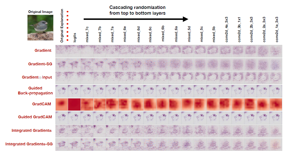
Here, each row corresponds to a different saliency map method. We see the saliency map explanations produced by the different methods as the CNN’s weights are progressively randomized from the top to the bottom layers. On the far right, complete randomization of all weights has been achieved, and we hope that the saliency map explanation has been destroyed.
Adebayo et al. emphasize that qualitative visual assessment of the saliency maps is not sufficient for understanding whether the saliency map has been destroyed. Thus, they provide a quantitative evaluation in Figures 3 and 4 (not shown) reporting the rank correlation, HOGs Similarity, and SSIM between the original saliency map and the randomized model saliency map. See the paper for details.
Sanity Check 2: Data Randomization Test
In the data randomization test, the model is trained on randomized training data, for which all training labels have been permuted – i.e. the model is trained on data for which there is no relationship between the data content and the data label. Perhaps an image of a dog is labeled “bird”, another image of a dog is labeled “plane”, and an image of a plane is labeled “person.”
Adebayo et al. explain the motivation for this test:
Our data randomization test evaluates the sensitivity of an explanation method to the relationship between instances and labels. An explanation method insensitive to randomizing labels cannot possibly explain mechanisms that depend on the relationship between instances and labels present in the data generating process.
The only way a neural network can do well on a task where the labels have been randomized is if the network memorizes the training dataset. In this sanity check, the models are trained until they have memorized enough of the training data to obtain greater than 95% training accuracy. However, their test accuracy is never better than random guessing, as they have not learned any generalizable principles (there are no generalizable principles to learn in a data set where the labels have been randomized.)
Finally, saliency map explanations are computed for all the examples in the test set, using the model just described (the one trained on randomly permuted labels) and a different model which was trained on the true labels. If the saliency map explanation relies at all on generalizable principles learned by the neural network to solve the task, then it should look different depending on whether the model was trained on true labels or randomized labels.
Sanity Check 2 Results:
- PASS/OKAY: Gradients, Gradient-SG, Grad-CAM
- FAIL: Guided Backpropagation, Guided GradCAM, Integrated Gradients, Gradient x Input
Here is the qualitative comparison of saliency maps shown in Figure 5:
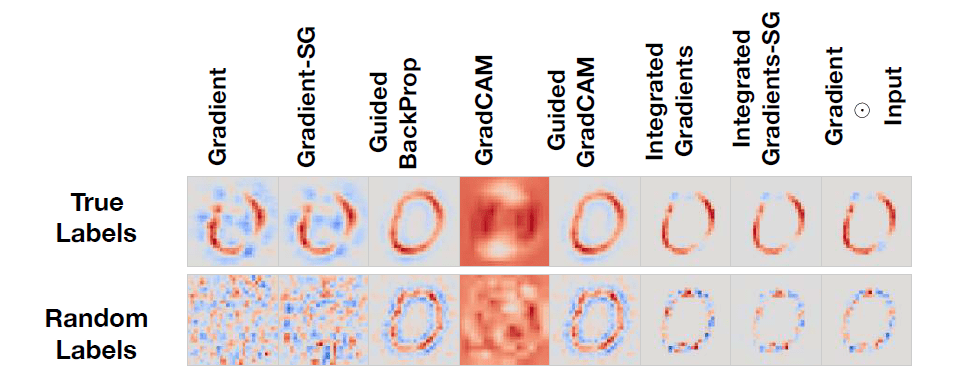
In this figure we can see the saliency map explanations for the digit 0 for a CNN trained on MNIST on true labels (top row) and random labels (bottom row.) For a saliency method that works, we’d expect the top row (“true labels”) to look good and the bottom row (“random labels”) to look terrible.
As before, it’s important not to rely solely on subjective visual assessment. Thus, the authors provide a quantitative comparison as well. In another piece of Figure 5, we can see the rank correlation between the saliency map of a model trained on true labels vs. the saliency map of a model trained on randomized labels:
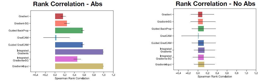
In this case, we want the rank correlation to be as close to 0 as possible. High values of rank correlation are bad because they mean that the saliency maps are similar between a model trained on true labels and a model trained on random labels. Note that “Abs” means we took the absolute value of the saliency map explanation while “No Abs” means we left the saliency map explanation as-is. We can see that Gradient has a low correlation in both cases (good), while Integrated Gradients has an extremely high correlation for the Abs case (bad).
Edge Detection
In the discussion, Adebayo et al. provide a case study of a 1-layer sum-pool CNN model. This case study suggests that some saliency methods may act like edge detectors because regions in the image corresponding to edges have a different activation pattern from the surrounding pixels, and thus will visually “stand out.” They note,
The human observer is at risk of confirmation bias when interpreting the highlighted edges as an explanation of the class prediction. […] In light of our findings, it is not unreasonable to interpret some saliency methods as implicitly implementing unsupervised image processing techniques, akin to edge detection.
Summary
If you’re using saliency map explanations in your work, stick to Gradients or plain GradCAM, as these methods appear to rely on the trained model’s weights and the relationship between training examples and their labels. It is likely best to avoid Guided Backpropagation and Guided GradCAM, as these approaches may merely be functioning as edge detectors rather than reliable explanations.
Featured Image
The featured image combines this Wikipedia image of The Thinker by Rodin with saliency maps from this repository.
Want to be the first to hear about my articles bridging healthcare, artificial intelligence, and business—and get a free list of my favorite health AI resources? Sign up here.

Comments are closed.