
In this post I will describe the CNN visualization technique commonly referred to as “saliency mapping” or sometimes as “backpropagation” (not to be confused with backpropagation used for training a CNN.) Saliency maps help us understand what a CNN is looking at during classification. For a summary of why that’s useful, see this post.
Saliency Map Example
The figure below shows three images — a snake, a dog, and a spider — and what the saliency maps look like for each image. Saliency maps are shown both in color and in grayscale. This figure is from utkuozbulak/pytorch-cnn-visualizations:
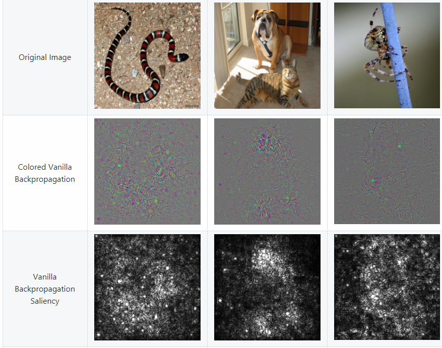
Above, “Colored Vanilla Backpropagation” means a saliency map created with RGB color channels. “Vanilla Backpropagation Saliency” is the result of converting the “Colored Vanilla Backpropagation” image into a grayscale image. You can see the code that was used to create these saliency maps at pytorch-cnn-visualizations/src/vanilla_backprop.py.
Definitions
Google defines “salient” as “most noticeable or important.” The concept of a “saliency map” is not limited to neural networks. A saliency map is any visualization of an image in which the most salient/most important pixels are highlighted. There are traditional computer vision saliency detection algorithms (e.g. OpenCV saliency API & tutorial). However, the focus of this post will be on saliency maps created from trained CNNs.
Paper Reference
If you’d like to read the paper that introduced saliency maps for CNNs, see Simonyan K, Vedaldi A, Zisserman A. Deep inside convolutional networks: Visualising image classification models and saliency maps. arXiv preprint arXiv:1312.6034. 2013 Dec 20. Cited by 1,479
The discussion of saliency maps begins on page 3, section 3 “Image-Specific Class Saliency Visualisation.” (This paper also includes a separate technique that creates a “canonical” image for each class.)
Recap of the Backpropagation Algorithm
The backpropagation algorithm allows neural networks to learn. Based on a training example, the backpropagation algorithm determines how much to increase or decrease each weight in a neural network in order to decrease the loss (i.e. in order to make the nerual network “less wrong”.) It does so by taking derivatives. After enough iterations of the neural network becoming “less wrong” as it sees many training examples, the network has become “mostly right” i.e. useful for solving the problem you asked it to solve. For a clear explanation of the backpropagation algorithm, see this post.
Saliency maps are sometimes referred to as “backpropagation” because they are visualizations of derivatives that are calculated using backpropagation. However, saliency maps are NOT used in training the network. Saliency maps are calculated after a network has finished training.
Purpose of Saliency Maps
The purpose of the saliency map approach is to query an already-trained classification CNN about the spatial support of a particular class in a particular image, i.e., “figure out where the cat is in the cat photo without any explicit location labels.”
Simple Linear Example
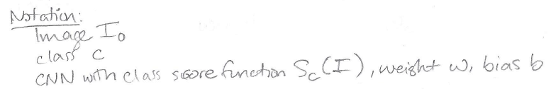
Simonyan et al. start out with a simple linear example that motivates saliency maps. First, some notation:
Using this notation, we can rephrase the purpose of saliency maps as follows:

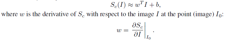
And finally, here is a summary of the simple linear example from Simonyan et al., in which each weight of a linear classification model indicates the importance of the corresponding image pixel in the classification task:
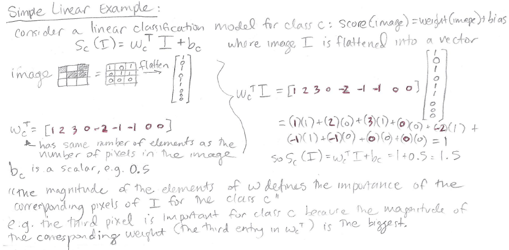
In essence, a weight with a bigger magnitude has more effect on the final classification score, and if the model is behaving reasonably then we’d expect the big-magnitude important weights to correspond to relevant parts of the image, e.g. correspond to the cat in a cat image.
CNN Example
Unfortunately, a CNN is a highly nonlinear scoring function, so the above simple linear example doesn’t directly apply. We can however still make use of similar reasoning by doing the following: let’s approximate the nonlinear scoring function of a CNN using a linear function in the neighborhood of the image. The authors frame this linear approximation as a first-order Taylor expansion:
Taylor Series Rabbit Hole
Per Wikipedia,
A Taylor series is a representation of a function as an infinite sum of terms that are calculated from the values of the function’s derivatives at a single point. […] The Taylor series of a real or complex-valued function f(x) that is infinitely differentiable at a real or complex number a is the power series

- Explanation of the numerator: Recall that the primes after the f‘s indicate the derivative. f is the function itself, f’ is the first derivative, f”’ is the third derivative, and f””””’ is the ninth derivative.
- Explanation of the denominator: Recall that an exclamation point after a number, e.g. 5!, indicates a factorial, which is calculated as e.g. 5! = 5 x 4 x 3 x 2 x 1.
- Connection to CNNs: in the case of a CNN, the function f() is the trained CNN itself, a is the particular image of interest, and x is a variable representing the CNN’s input, i.e. an arbitrary image.
A Taylor series is cool because it implies that if you know the value of a function and the function’s derivatives at a certain point, then you can use a Taylor series approximation to estimate the value of that function at any other point. For instance you might know the value of the function and its derivatives at a = 6, so you can use a Taylor series approximation to estimate the value of the function at x = 10,369.
After thinking about Taylor series in the context of this paper, I am not convinced that the best way to understand saliency maps is by thinking about Taylor series. In case it helps anyone else, I am putting my thoughts here:
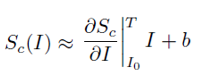
The paper says they’re using a “first-order Taylor expansion” which technically should be this:

i.e. including f(a) which in this case would be the CNN applied to our particular image of interest. However in the actual implementation of saliency maps, it does not appear that the calculated output of the CNN, f(a), is used at all. Rather, only the first-order derivative piece is used:
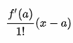
and even there, only the piece f'(a)(x) is focused on in their explanation:
where a = I_zero, f'(a) is the derivative  , and x is I.
Furthermore, in practice, only the derivative piece is actually used to make the saliency map! The derivative piece IS the saliency map:
i.e., the saliency map is a visual representation of the derivative of the score with respect to the image variable, evaluated at the point (particular image) I_zero.
Thinking about Saliency Maps
Why should we want to compute the derivative of the score with respect to an image? The authors explain,
Another interpretation of computing the image-specific class saliency using the class score derivative is that the magnitude of the derivative indicates which pixels need to be changed the least to affect the class score the most. One can expect that such pixels correspond to the object location in the image.
So if we have an image of a cat that has a high score for the class “cat” we want to know which pixels in the cat image were important for computing the high score for class “cat.” We take the derivative of the score for class “cat” with respect to our particular cat image. The pixels with large-magnitude derivatives are pixels that have a large influence on the score for class “cat” so, unless the neural network is “cheating” and looking at non-cat cues in the image to classify “cat”, these important pixels correspond to the location of the cat. Thus, saliency maps enable a form of weakly-supervised object localization: we can get approximate locations of objects from a model that was trained only on class labels.
Steps for Computing a Saliency Map
(ref: top of page 4 in the paper)
(1) Find the derivative of the score with respect to the image.
(2) For an image composed of m x n pixels, the derivative is an m x n matrix. Take the absolute value of each element of the derivative matrix.
(3) If you have a three-channel color image (RGB) take the maximum of the three color channel derivative values at each pixel.
(3) Plot the absolute-valued derivative matrix as if it’s an image, and that’s your saliency map.
Here’s Pytorch code for computing a saliency map. It’s missing an explicit “absolute value” step, but the result should look somewhat visually similar.
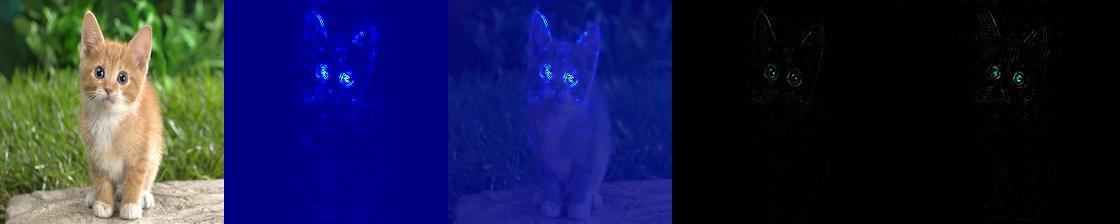
Here’s Tensorflow code (source of the cat image below); in the code you can see step (2), the absolute value of the derivative matrix, at line 83.
You can see more visualizations of saliency maps on pages 5 and 6 of the paper (Figures 2 and 3).
Conclusion
Saliency maps can be used to highlight the approximate location of an object in an image. A saliency map is the derivative of the class score with respect to the input image.
Saliency maps are the precursor to guided saliency/guided backpropagation, which in turn is used in Guided Grad-CAM. Both of these techniques will be topics of future posts.
About the Featured Image
The featured image is a rabbit, Oryctolagus cuniculus. The phrase “down the rabbit hole” comes from the children’s book Alice’s Adventures in Wonderland by Lewis Carrol.
Want to be the first to hear about my articles bridging healthcare, artificial intelligence, and business—and get a free list of my favorite health AI resources? Sign up here.

Comments are closed.