Convolution vs. Cross-Correlation

This post will overview the difference between convolution and cross-correlation. This post is the only resource online that contains a step-by-step worked example of both convolution and cross-correlation together (as far as I know – and trust me, I did a lot of searching). This post also deals precisely with indices, which it turns out are critical to get right if you want to demonstrate by example how convolution and cross-correlation are related. I spent a large part of preparing this post tearing my hair out over indices, but now they are all beautiful and organized for you to enjoy.

First, a little motivation on this topic…

Motivation

It is necessary to understand the difference between convolution and cross-correlation in order to understand backpropagation in CNNs, which is necessary to understand deconvnets (a CNN visualization technique), which is necessary to understand the difference between deconvnets and saliency maps (more visualization), which is necessary to understand guided backpropagation (more visualization), which is necessary to understand Grad-CAM (more visualization), which is necessary to understand Guided Attention Inference Networks (a method built off of Grad-CAM that includes a new way to train attention maps). So, although “convolution vs. cross-correlation” may initially appear off-topic, this article is actually still part of the series on CNN heat maps.

For a review of CNNs, please see Intro to Convolutional Neural Networks.

Now that you are highly motivated, let’s dive in!

High-Level Summary

Cross-correlation and convolution are both operations applied to images. Cross-correlation means sliding a kernel (filter) across an image. Convolution means sliding a flipped kernel across an image. Most convolutional neural networks in machine learning libraries are actually implemented using cross-correlation, but it doesn’t change the results in practice because if convolution were used instead, the same weight values would be learned in a flipped orientation.

Keeping Track of Indices

In order for the convolution and cross-correlation examples and equations to be clear we need to keep track of our image indices, kernel indices, and output indices.

First, here’s a figure that’s popularly used to explain convolution, in which a kernel (yellow) slides across an image (green) to produce an output (pink):

(Image Source: This animation appears in many places, including here and here.)

When we index into the image, what pixel do we call [0,0]? We could choose the upper left-hand corner, or the center, or some other arbitrary pixel. Similarly, what do we call [0,0] in the kernel or the output?

For the image, the kernel, and the output, we will call the center element [0,0]. This decision is important in order to make the formulas work out nicely.

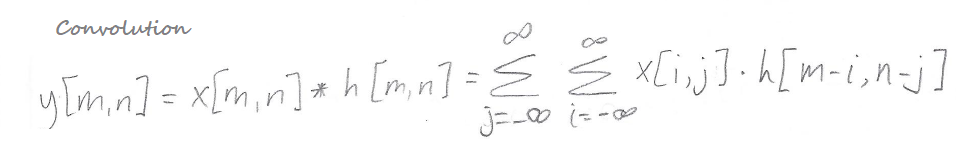
Convolution Setup: Notation & Equation

There are a LOT of equations for convolution floating around on the web, all with different notation and indexing. For example:

For the remainder of this post we will be using the following notation, in which the image is referred to as x, the kernel as h, and the output as y:

This is the notation used by Song Ho Ahn in their helpful post on 2D convolution.

The star * is used to denote the convolution operation. Thus, x[m,n]*h[m,n] means we are convolving an image x with a kernel h to find the value that goes in the output y at position [m, n]. The sums are over i and j, which index into the image pixels.

Here’s a drawing of the kernel (filter), in which we see the center of the kernel is [0,0] as we decided before. m (red) indexes horizontally into columns, and n (green) indexes vertically into rows of the kernel:

The indices of the kernel elements are shown on the left, in red and green. The actual kernel numeric values are represented as the variables a, b, c, d, e, f, g, h, and i, shown on the right. (These numeric values in the kernel are what a CNN learns during the process of training.)

Finally, here’s the 7-by-7 image x, indexed from -3 to 3:

Here’s the lower right-hand corner of image x, zoomed in because this is the piece of the image we’re going to focus on in the worked example:

For this piece of the image, I wrote out the indexes of each of the pixels. These are not the pixel values – they are just the [i, j] coordinates of each pixel. You can imagine this image having arbitrary pixel values, because we’re not going to need the image pixel values in our example.

Convolution Example (Math)

Recall the equation for convolution:

What this initially seems to suggest is that in order to obtain the value at index [m,n] in the output y, we need to look at all of the pixels in the image. After all, i and j are indexing into the image, and the sums go across values of i and j from minus infinity to positive infinity.

However, in actuality, we aren’t going to need all the pixels, because for particular output indices m and n, choosing certain pixel indices i and j will lead to accessing kernel elements that don’t exist. So, we are only going to end up looking at the pixels of the image for which the kernel part of the equation h[m-i,n-j] is still valid. To illustrate this effect, in the below example I’ve included the pixel indices i = 3 and j = 3; you can see that for the chosen output element y[m=1,n=1], choosing i = 3 or j = 3 leads to an attempted access of a kernel element which doesn’t exist (e.g. kernel element (1,2); refer to the picture of the kernel from earlier and you’ll see its indices only go from -1 to +1). Thus, we are not explicitly saying which image indices i and j are needed for each part of the output map; it’s implicit in the formula, based on what choices of i and j will lead to acceptable kernel accesses.

(Note that instead of summing from “minus infinity to positive infinity” which is a little weird since no picture has infinite size, we could instead write “-k to +k” but that has the drawback of implying a fixed k x k input image size.)

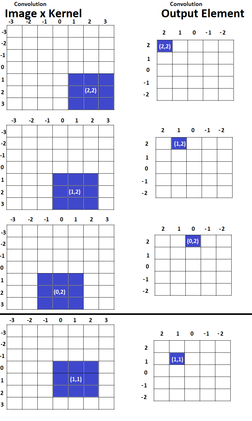
Without further ado, here’s the worked example of convolution to produce the output entry y[m=1,n=1]:

What is happening here?

Well, first of all, we are trying to find the value at a single place in the output map y, specified by the indices m = 1, n = 1; we want to find y[1,1]. For simplicity I didn’t show every single possible combination of pixel values i and j (from -3 to +3), because that would’ve gotten really cluttered and all of the ones I didn’t show are “invalid” (i.e. they need kernel indices that don’t exist.)

There’s a blue line going down the center of the image. On the left of the blue line, we have the values of m, n, i, and j plugged straight in to the convolution equation in a systematic way. On the right of the blue line, we have “solved” the expression on the left, to get the final indices of h[#,#] that we multiply against that particular pixel x[#,#].

Convolution Example (Drawing)

The equations above might seem like a lot of mumbo-jumbo, but if we organize them into a picture, we can suddenly see why they are cool. In the picture below, I show the lower right-hand corner of the image x with the relevant pixel indices written out explicitly. Then I’ve lined up the kernel h against the image in the relevant spot, and I’ve used the result of the convolution equation to fill in the kernel indices h[#,#] so that the right h[#,#] goes with the right x[#,#]. Finally, I’ve referenced the original kernel picture (earlier in the post) to figure out which kernel numeric values (a, b, c, etcetera) correspond to which kernel indices…and VOILA!!! We have shown that convolution “flips the kernel”:

So, if you ever read anything about how “real convolution uses a flipped kernel” now you understand why, in math.

Cross-Correlation Compared to Convolution

Cross-correlation may be what you think of when you think of “convolution,” because cross-correlation means sliding a kernel across an image without flipping the kernel. Here are the equations for cross-correlation and convolution side-by-side, so you can compare them:

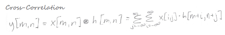
As you can see, the key difference is a plus sign versus a minus sign in the expression h[m-i, n-j] or h[m+i, n+j]. That one difference ends up determining (a) whether the kernel is flipped and (b) what pixels are processed for each element of the output map.

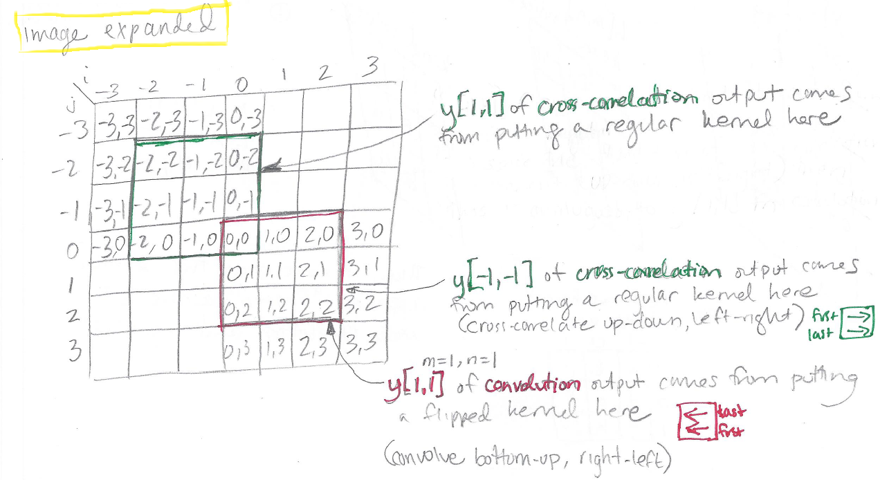
In the figure above, we can see the following:

• In order to obtain the output value at y[m=1,n=1] for cross-correlation we need to look at the pixels that are boxed in green (because these are the only pixels for which the kernel indices make sense.)
• However, to obtain the output value at y[m=1,n=1] for convolution, we need to look at a different set of pixels, boxed in red (because these are now the only pixels for which the kernel indices make sense.)
• It turns out that if we want to do a single worked example using the same piece of the input image, this same piece of the input image corresponds to different pieces of the output map for convolution and cross-correlation. That’s because convolution takes place starting in the bottom right corner and going bottom-up/right-left, while cross-correlation takes place starting in the upper left corner and going top-down/left-right. Thus, the part of the image we are focused on – the part boxed in red – corresponds to convolution output y[1,1] but to cross-correlation output y[-1,-1].

As a further summary of the matter, here are two figures showing what part of the input image is used to create different parts of the output map, for cross-correlation vs. convolution:

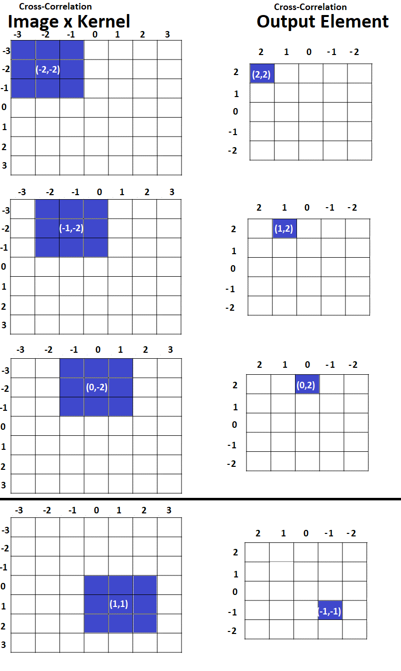
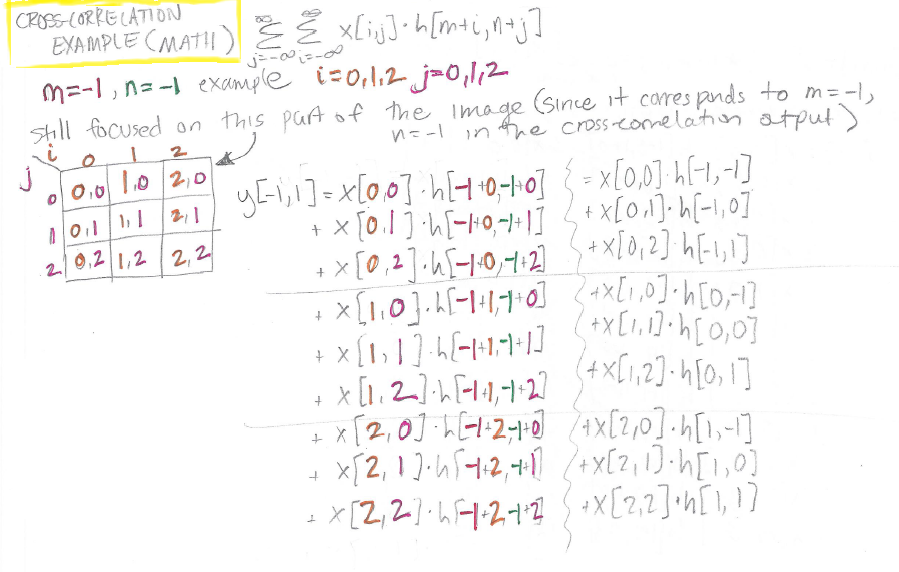
Cross-Correlation Example (Math)

Finally, with that background, here’s our worked example for the “red patch” of the image that we’re focused on. In cross-correlation, this patch is used to find the output at y[m= -1, n= -1]:

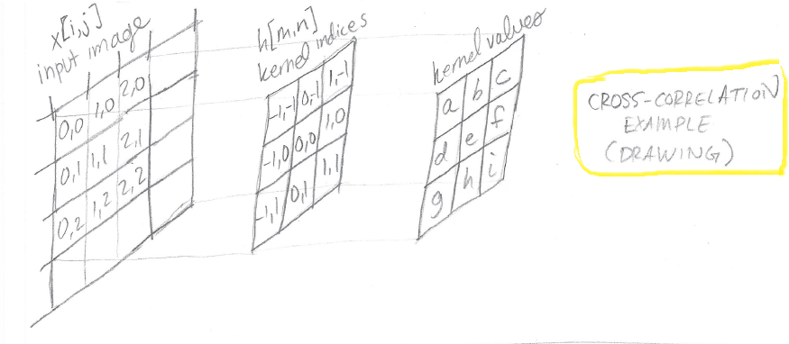
Cross-Correlation Example (Drawing)

Once again, we can use the math above to fill in a picture showing us what is happening at the level of the image and the kernel. We can see by lining up the appropriate kernel indices with the input image indices that we end up with the kernel “facing the original direction” i.e. in cross-correlation the kernel is not flipped.

Summary

• Convolution and cross-correlation both involve sliding a kernel across an image to create an output.
  • In convolution, the kernel is flipped
  • In cross-correlation, the kernel is not flipped
  • Most animations and explanations of convolution are actually presenting cross-correlation, and most implementations of “convolutional neural networks” actually use cross-correlation. In a machine learning context this doesn’t change the model’s performance because the CNN weights are just learned flipped.
• To make the formulas work out nicely in an example, you need to:
  • (1) Choose the indices appropriately. The center element of the image, kernel, and output are each [0,0]
  • (2) Be aware that a fixed patch of the image corresponds to different indices of the output map in convolution vs. cross-correlation. This occurs because in convolution the kernel traverses the image bottom-up/right-left, while in cross-correlation, the kernel traverses the image top-down/left-right.
• Understanding the difference between convolution and cross-correlation will aid in understanding how backpropagation works in CNNs, which is the topic of a future post.

References

• Convolution vs. Cross Correlation, video from Udacity “Computational Photography” (also, all of Lesson 10, a video series with examples, animations, and formulas)
• Deep Learning Book Chapter 9 (summary formulas)
• CENG 793 Akbas Week 3 CNNs and RNNs (summary formulas)
• Example of 2D Convolution by Song Ho Ahn (example with indices)
• Convolution by Song Ho Ahn (example with indices)

About the Featured Image

Image Source: Peggy Bacon in mid-air backflip. Remember…real convolution flips the kernel.