
Convolutional neural networks (CNNs) are the most popular machine leaning models for image and video analysis.
Example Tasks
Here are some example tasks that can be performed with a CNN:
- Binary Classification: given an input image from a medical scan, determine if the patient has a lung nodule (1) or not (0)
- Multilabel Classification: given an input image from a medical scan, determine if the patient has none, some, or all of the following: lung opacity, nodule, mass, atelectasis, cardiomegaly, pneumothorax
How CNNs Work
In a CNN, a convolutional filter slides across an image to produce a feature map (which is labeled “convolved feature” in the image below):
A filter detects a pattern.
High values in the output feature map are produced when the filter passes over an area of the image containing the pattern.
Different filters detect different patterns.
The kind of pattern that a filter detects is determined by the filter’s weights, which are shown as red numbers in the animation above.
A filter weight gets multiplied against the corresponding pixel value, and then the results of these multiplications are summed up to produce the output value that goes in the feature map.
A convolutional neural network involves applying this convolution operation many time, with many different filters.
This figure shows the first layer of a CNN:

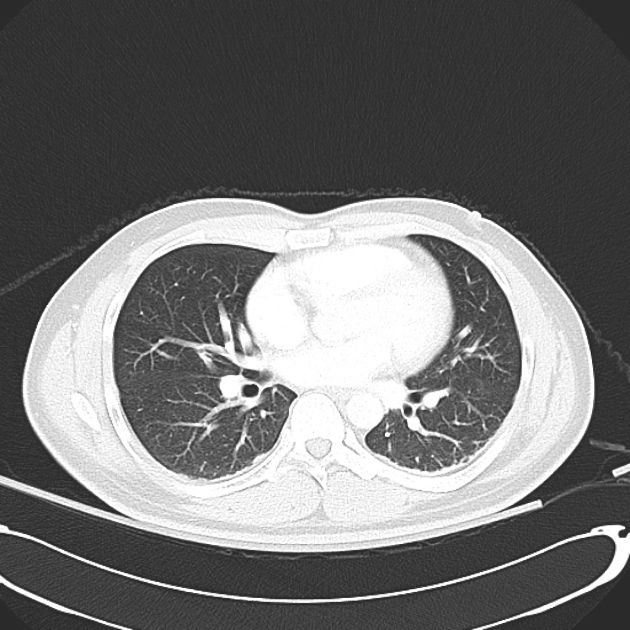
In the diagram above, a CT scan slice (slice source: Radiopedia) is the input to a CNN. A convolutional filter labeled “filter 1” is shown in red. This filter slides across the input CT slice to produce a feature map, shown in red as “map 1.”
Then a different filter called “filter 2” (not explicitly shown) which detects a different pattern slides across the input CT slice to produce feature map 2, shown in purple as “map 2.”
This process is repeated for filter 3 (producing map 3 in yellow), filter 4 (producing map 4 in blue) and so on, until filter 8 (producing map 8 in red).
This is the “first layer” of the CNN. The output of the first layer is thus a 3D chunk of numbers, consisting in this example of 8 different 2D feature maps.

Next we go to the second layer of the CNN, which is shown above. We take our 3D representation (of 8 feature maps) and apply a filter called “filter a” to this. “Filter a” (in gray) is part of the second layer of the CNN. Notice that “filter a” is actually three dimensional, because it has a little 2×2 square of weights on each of the 8 different feature maps. Therefore the size of “filter a” is 8 x 2 x 2. In general, the filters in a “2D” CNN are 3D, and the filters in a “3D” CNN are 4D.
We slide filter a across the representation to produce map a, shown in grey. Then, we slide filter b across to get map b, and filter c across to get map c, and so on. This completes the second layer of the CNN.
We can then continue on to a third layer, a fourth layer, etc. for however many layers of the CNN are desired. CNNs can have many layers. As an example, a ResNet-18 CNN architecture has 18 layers.
The figure below, from Krizhevsky et al., shows example filters from the early layers of a CNN. The filters early on in a CNN detect simple patterns like edges and lines going in certain directions, or simple color combinations.

The figure below, from Siegel et al. adapted from Lee et al., shows examples of early layer filters at the bottom, intermediate layer filters in the middle, and later layer filters at the top.
The early layer filters once again detect simple patterns like lines going in certain directions, while the intermediate layer filters detect more complex patterns like parts of faces, parts of cars, parts of elephants, and parts of chairs. The later layer filters detect patterns that are even more complicated, like whole faces, whole cars, etc. In this visualization each later layer filter is visualized as a weighted linear combination of the previous layer’s filters.

How to Learn the Filters
How do we know what feature values to use inside of each filter? We learn the feature values from the data. This is the “learning” part of “machine learning” or “deep learning.”
Steps:
- Randomly initialize the feature values (weights). At this stage, the model produces garbage — its predictions are completely random and have nothing to do with the input.
- Repeat the following steps for a bunch of training examples: (a) Feed a training example to the model (b) Calculate how wrong the model was using the loss function (c) Use the backpropagation algorithm to make tiny adjustments to the feature values (weights), so that the model will be less wrong next time. As the model becomes less and less wrong with each training example, it will ideally learn how to perform the task very well by the end of training.
- Evaluate model on test examples it’s never seen before. The test examples are images that were set aside and not used in training. If the model does well on the test examples, then it’s learned generalizable principles and is a useful model. If the model does badly on the test examples, then it’s memorized the training data and is a useless model.
The following animation created by Tamas Szilagyi shows a neural network model learning. The animation shows a feedforward neural network rather than a convolutional neural network, but the learning principle is the same. In this animation each line represents a weight. The number shown next to the line is the weight value. The weight value changes as the model learns.

Measuring Performance: AUROC

One popular performance metric for CNNs is the AUROC, or area under the receiver operating characteristic. This performance metric indicates whether the model can correctly rank examples. The AUROC is the probability that a randomly selected positive example has a higher predicted probability of being positive than a randomly selected negative example. An AUROC of 0.5 corresponds to a coin flip or useless model, while an AUROC of 1.0 corresponds to a perfect model.
Additional Reading
For more details about CNNs, see:
- How Computers See: Intro to Convolutional Neural Networks
- The History of Convolutional Neural Networks
- Convolution vs. Cross-Correlation
For more details about how neural networks learn, see Introduction to Neural Networks.
Finally, for more details about AUROC, see:
- Measuring Performance: AUC (AUROC)
- The Complete Guide to AUC and Average Precision: Simulations nad Visualizations
Want to be the first to hear about my articles bridging healthcare, artificial intelligence, and business—and get a free list of my favorite health AI resources? Sign up here.

Comments are closed.