
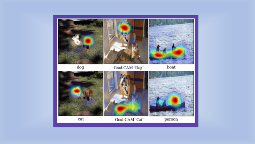
Grad-CAM is a popular technique for visualizing where a convolutional neural network model is looking. Grad-CAM is class-specific, meaning it can produce a separate visualization for every class present in the image:

Example cat and dog Grad-CAM visualizations modified from Figure 1 of the Grad-CAM paper
Grad-CAM can be used for weakly-supervised localization, i.e. determining the location of particular objects using a model that was trained only on whole-image labels rather than explicit location annotations.
Grad-CAM can also be used for weakly-supervised segmentation, in which the model predicts all of the pixels that belong to particular objects, without requiring pixel-level labels for training:
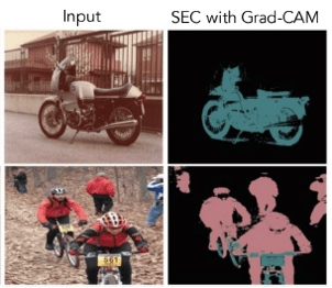
Part of Figure 4 of the Grad-CAM paper showing predicted motorcycle and person segmentation masks obtained by using Grad-CAM heatmaps as the seed for a method called SEC (Seed, Expand, Constrain)
Finally, Grad-CAM can be used to gain better understanding of a model, for example by providing insight into model failure modes:
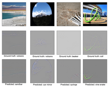
Figure 6 of the Grad-CAM paper, showing example model failures along with Grad-CAM visualizations that illustrate why the model made incorrect predictions.
The main reference for this post is the expanded version of the Grad-CAM paper: Selvaraju et al. “Grad-CAM: Visual Explanations from Deep Networks via Gradient-based Localization.” International Journal of Computer Vision 2019.
A previous version of the Grad-CAM paper was published in the International Conference on Computer Vision (ICCV) 2017.
Update in 2021
While the Grad-CAM paper has been cited several thousand times, recent work demonstrates a serious problem with Grad-CAM: sometimes, Grad-CAM highlights regions of an image that a model did not actually use for prediction. This means Grad-CAM is an unreliable model explanation method. HiResCAM is a new explanation method that is provably guaranteed to highlight only locations the model used. HiResCAM is inspired by Grad-CAM, so if you understand Grad-CAM, it’s straightforward to then understand how HiResCAM works.
Grad-CAM as Post-Hoc Attention
Grad-CAM is a form of post-hoc attention, meaning that it is a method for producing heatmaps that is applied to an already-trained neural network after training is complete and the parameters are fixed. This is distinct from trainable attention, which involves learning how to produce attention maps (heatmaps) during training by learning particular parameters. For a more in-depth discussion of post-hoc vs. trainable attention, see this post.
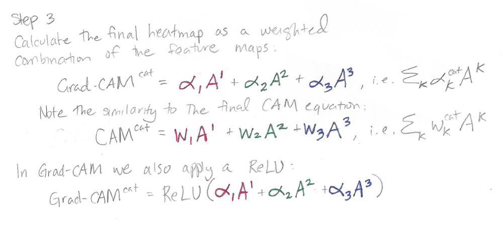
Grad-CAM as a Generalization of CAM
Grad-CAM does not require a particular CNN architecture. Grad-CAM is a generalization of CAM (class activation mapping), a method that does require using a particular architecture.
CAM requires an architecture that applies global average pooling (GAP) to the final convolutional feature maps, followed by a single fully connected layer that produces the predictions:
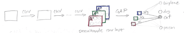
In the sketch above, the squares A1 (red), A2 (green), and A3 (blue) represent feature maps produced by the last convolutional layer of a CNN. To use the CAM method upon which Grad-CAM is based, we first take the average of each feature map to produce a single number per map. In this example we have 3 feature maps and therefore 3 numbers; the 3 numbers are shown as the tiny colored squares in the sketch. Then we apply a fully-connected layer to those 3 numbers obtain classification decisions. For the output class “cat” the prediction will be based on 3 weights (w1, w2, and w3). To make a CAM heatmap for “cat”, we perform a weighted sum of the feature maps, using the “cat” weights of the final fully-connected layer:

Note that the number of feature maps doesn’t have to be three – it an be any arbitrary k. For a more detailed explanation of how CAM works, please see this post. Understanding CAM is important for understanding Grad-CAM, as the two methods are closely related.
Part of the motivation for the development of Grad-CAM was to come up with a CAM-like method that does not restrict the CNN architecture.
Grad-CAM Overview
The basic idea behind Grad-CAM is the same as the basic idea behind CAM: we want to exploit the spatial information that is preserved through convolutional layers, in order to understand which parts of an input image were important for a classification decision.
Similar to CAM, Grad-CAM uses the feature maps produced by the last convolutional layer of a CNN. The authors of Grad-CAM argue, “we can expect the last convolutional layers to have the best compromise between high-level semantics and detailed spatial information.”
Here is a sketch showing the parts of a neural network model relevant to Grad-CAM:
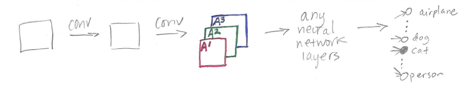
The CNN is composed of some convolutional layers (shown as “conv” in the sketch). The feature maps produced by the final convolutional layer are shown as A1, A2, and A3, the same as in the CAM sketch.
At this point, for CAM we would need to do global average pooling followed by a fully connected layer. For Grad-CAM, we can do anything – for example, multiple fully connected layers – which is shown as “any neural network layers” in the sketch. The only requirement is that the layers we insert after A1, A2, and A3 have to be differentiable so that we can get a gradient. Finally, we have our classification outputs for airplane, dog, cat, person, etc.
The difference between CAM and Grad-CAM is in how the feature maps A1, A2, and A3 are weighted to make the final heatmap. In CAM, we weight these feature maps using weights taken out of the last fully-connected layer of the network. In Grad-CAM, we weight the feature maps using “alpha values” that are calculated based on gradients. Therefore, Grad-CAM does not require a particular architecture, because we can calculate gradients through any kind of neural network layer we want. The “Grad” in Grad-CAM stands for “gradient.”
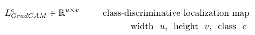
The output of Grad-CAM is a “class-discriminative localization map”, i.e. a heatmap where the hot part corresponds to a particular class:

If there are 10 possible output classes, then for a particular input image, you can make 10 different Grad-CAM heatmaps, one heatmap for each class.
Grad-CAM Details
First, a bit of notation:
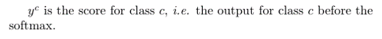
In other words, y^c is the raw output of the neural network for class c, before the softmax is applied to transform the raw score into a probability.
Grad-CAM is applied to a neural network that is done training. The weights of the neural network are fixed. We feed an image into the network to calculate the Grad-CAM heatmap for that image for a chosen class of interest.
Grad-CAM has three steps:
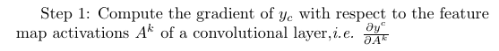
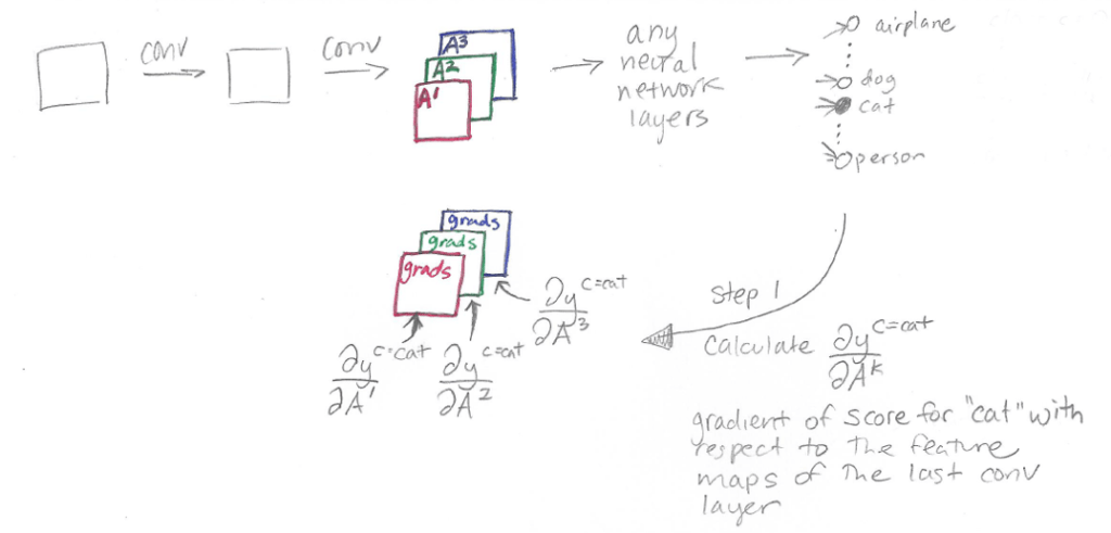
Step 1: Compute Gradient
The particular value of the gradient calculated in this step depends on the input image chosen, because the input image determines the feature maps A^k as well as the final class score y^c that is produced.
For a 2D input image, this gradient is 3D, with the same shape as the feature maps. There are k feature maps each of height v and width u, i.e. collectively the feature maps have shape [k, v, u]. This means that the gradients calculated in Step 1 are also going to be of shape [k, v, u].
In the sketch below, k=3 so there are three u x v feature maps and three u x v gradients:
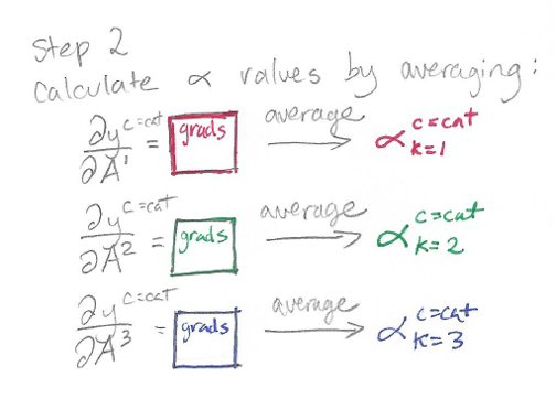
Step 2: Calculate Alphas by Averaging Gradients
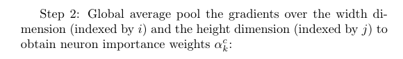
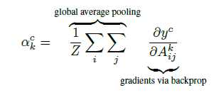
In this step, we calculate the alpha values. The alpha value for class c and feature map k is going to be used in the next step as a weight applied to the feature map A^k. (In CAM, the weight applied to the feature map A^k is the weight w_k in the final fully connected layer.)
Recall that our gradients have shape [k, v, u]. We do pooling over the height v and the width u so we end up with something of shape [k, 1, 1] or to simplify, just [k]. These are our k alpha values.
Step 3: Calculate Final Grad-CAM Heatmap
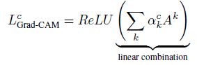
Now that we have our alpha values, we use each alpha value as the weight of the corresponding feature map, and calculate a weighted sum of feature maps as the final Grad-CAM heatmap. We then apply a ReLU operation to emphasize only the positive values and turn all the negative values into 0.
Won’t the Grad-CAM Heatmap Be Too Small?
The Grad-CAM heatmap is size u x v, which is the size of the final convolutional feature map:
You may wonder how this makes sense, since in most CNNs the final convolutional features are quite a bit smaller in width and height than the original input image.
It turns out it is okay if the u x v Grad-CAM heatmap is a lot smaller than the original input image size. All we need to do is up-sample the tiny u x v heatmap to match the size of the original image before we make the final visualization.
For example, here is a small 12 x 12 heatmap:
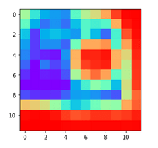
Now, here is the same heatmap upsampled to 420 x 420 using the Python package cv2:
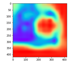
The code to visualize the original small low-resolution heatmap and turn it into a big high-resolution heatmap is here:
import cv2
import matplotlib
import matplotlib.pyplot as plt

small_heatmap = CalculateGradCAM(class='cat')

plt.imshow(small_heatmap, cmap='rainbow')

#Upsample the small_heatmap into a big_heatmap with cv2:
big_heatmap = cv2.resize(small_heatmap, dsize=(420, 420),
                         interpolation=cv2.INTER_CUBIC)

plt.imshow(big_heatmap, cmap='rainbow')
Grad-CAM Implementation
A Pytorch implementation of Grad-CAM is available here.
More Grad-CAM Examples
Grad-CAM has been applied in numerous research areas and is particularly popular in medical images. Here are a few examples:

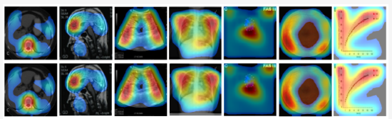
Top row is CAM, bottom row is Grad-CAM. Kim et al. “Visual Interpretation of Convolutional Neural Network Predictions in Classifying Medical Image Modalities.”
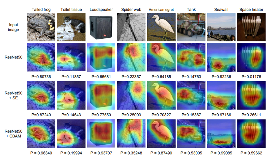
Grad-CAM visualizations from Woo et al. “CBAM: Convolutional Block Attention Module.” This paper is an example of a trainable attention mechanism (CBAM) combined with a post-hoc attention mechanism for visualization (Grad-CAM).
Major Issue with Grad-CAM identified in 2021
Although Grad-CAM is supposed to be able to explain what regions of an image a model used for prediction, it turns out that Grad-CAM is not guaranteed to do this! In brief, because of the gradient averaging step, Grad-CAM’s heat maps do not reflect the model’s computations and thus can highlight irrelevant areas that weren’t used for prediction. The solution is HiResCAM, an explanation method that avoids Grad-CAM’s gradient averaging step and instead uses an element-wise product between the raw gradients and the feature maps. HiResCAM accomplishes all the same purposes as Grad-CAM, with the benefit that HiResCAM is provably guaranteed to highlight only the regions the model used, for any CNN ending in one fully connected layer. It takes only a few seconds to change Grad-CAM code into HiResCAM code. For more details on why Grad-CAM sometimes fails, and how the HiResCAM solution works, see this paper.
Problems with Guided Grad-CAM
As another issue to be aware of, the Grad-CAM paper mentions a variant of Grad-CAM called “Guided Grad-CAM” which combines Grad-CAM with another CNN heatmap visualization technique called “guided backpropagation.” I discuss guided backpropagation in this post and this post. The short summary is that recent work by Adebayo et al. and Nie et al. suggests that guided backpropagation is performing partial image recovery and acting like an edge detector, rather than providing insight into a trained model. Therefore, it is best not to use guided backpropagation, and by extension this means it’s best not to use Guided Grad-CAM.
Summary
- Grad-CAM is a popular technique for creating a class-specific heatmap based off of a particular input image, a trained CNN, and a chosen class of interest.
- Grad-CAM is closely related to CAM.
- Grad-CAM can be calculated on any CNN architecture as long the layers are differentiable.
- Grad-CAM has been used for weakly-supervised localization and weakly-supervised segmentation.
- Recent work identifies a fundamental problem with Grad-CAM: sometimes Grad-CAM highlights regions the model did not actually use. Thus, for model explanation, HiResCAM should be used instead of Grad-CAM.
About the Featured Image
The featured image is modified from Figures 1 and 20 of the Grad-CAM paper.
Want to be the first to hear about my articles bridging healthcare, artificial intelligence, and business—and get a free list of my favorite health AI resources? Sign up here.

Comments are closed.