Comparing AUCs of Machine Learning Models with DeLong’s Test

Have you ever wondered how to demonstrate that one machine learning model’s test set performance differs significantly from the test set performance of an alternative model? This post will describe how to use DeLong’s test to obtain a p-value for whether one model has a significantly different AUC than another model, where AUC refers to the area under the receiver operating characteristic. This post includes a hand-calculated example to illustrate all the steps in DeLong’s test for a small data set. It also includes an example R implementation of DeLong’s test to enable efficient calculation on large data sets.

An example use case for DeLong’s test: Model A predicts heart disease risk with AUC of 0.92, and Model B predicts heart disease risk with AUC of 0.87, and we use DeLong’s test to demonstrate that Model A has a significantly different AUC from Model B with p < 0.05.

References

Elizabeth Ray DeLong is a statistician and professor at Duke University. In 1988 she published a test for determining whether the AUCs of two models are statistically  significantly different. This test has come to be known as “DeLong’s test.”

The main references for this post are:

• Elizabeth DeLong et al. “Comparing the Areas under Two or More Correlated Receiver Operating Characteristic Curves: A Nonparametric Approach.” Biometrics 1988.
• Xu Sun et al. “Fast Implementation of DeLong’s Algorithm for Comparing the Areas Under Correlated Receiver Operating Characteristic Curves.” IEEE Signal Processing Letters 2014. 

Conveniently, both papers use similar notation, which is the notation we will use in this post.

Definitions of Sensitivity and Specificity

To understand how DeLong’s test works, we need to start with some notation. We will get used to this notation by using it to define sensitivity, specificity, and AUC.

Consider a situation in which we have built a model to predict whether or not an individual has a disease. We make predictions on a test data set of N patients total, of which m are truly diseased and n are truly healthy. Our model produces predicted probabilities X for the m diseased patients, and predicted probabilities Y for the n healthy patients:

Using this notation, we can write out the definitions for sensitivity and specificity:

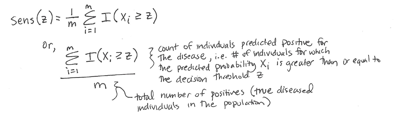
Sensitivity is also known as recall or true positive rate. It is the proportion of true positives (diseased people) that are correctly identified as positives (diseased) by the model. We define the sensitivity at a certain decision threshold z as follows:

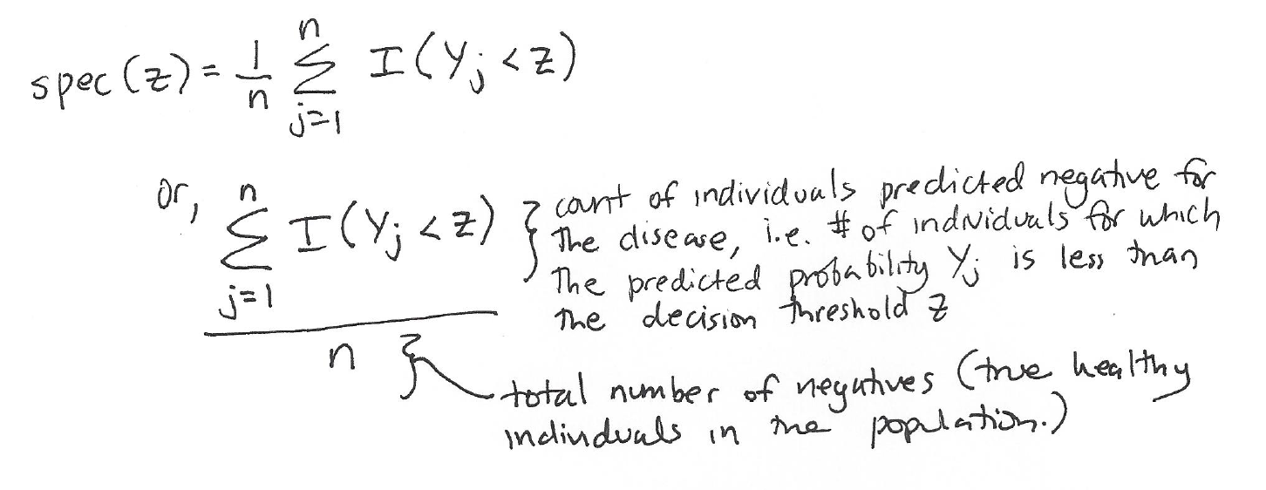
Specificity is also known as the true negative rate. It is the proportion of true negatives (healthy people) that are correctly identified as negatives (healthy) by the model. We define specificity at a certain decision threshold z as follows:

This means that as we vary the decision threshold z, we will vary the sensitivity and the specificity.

Definition of AUC and Calculation of Empirical AUC

The receiver operating characteristic (ROC) provides a summary of the sensitivity and specificity across different thresholds z. We build a ROC curve by varying the threshold z and plotting the sensitivity versus (1 – specificity) at each z value.

The area under the ROC curve, or AUC, provides a single number to summarize of the model’s performance across all the different decision thresholds.

In the paper, DeLong et al. describe a method in which an empirical AUC “is calculated by summing the area of trapezoids that are formed below the connected points making up the ROC curve” (ref).

For context, DeLong’s empirical AUC approach is different from a binomial AUC approach. A binomial ROC curve is constructed “based on the assumption that the diagnostic test scores corresponding to the positive condition and the scores corresponding to the negative condition can each be represented by a normal distribution” (ref).

The empirical AUC approach is more popular than the binomial AUC approach because the empirical AUC does not rely on the strong normality assumptions that the binomial AUC requires.

We can calculate the empirical AUC (represented as “theta hat”) with the trapezoid rule as follows:

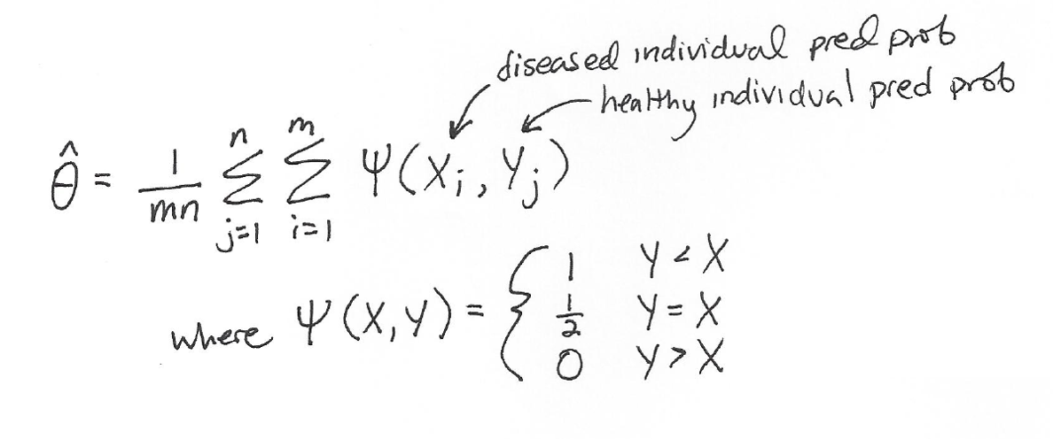
This definition of AUC makes intuitive sense:

• When Y < X, this means that the predicted disease probability of a healthy individual is less than the predicted disease probability of a sick individual, which is good: we want actually healthy people to have lower predicted disease risk than actually sick people. So, we reward the model for its good prediction and make a contribution to the model’s AUC of +1/mn.
• When Y = X, this means that the predicted disease probability of a healthy individual is equal to the predicted disease probability of a sick individual, which isn’t awesome but isn’t horrible, so we make a contribution to the model’s AUC of (+1/2)/mn.
• When Y > X, this means that the predicted disease probability of a healthy individual is greater than the predicted disease probability of a sick individual, which is bad: the model thought that an actually healthy person had higher disease risk than an actually sick person. We don’t add anything to the model’s AUC here (+0).

The function psi(X,Y) is also known as the Heaviside function (with the half-maximum convention).

For additional background on sensitivity, specificity, and how to construct a ROC curve, please see this post.

Connection between AUC and the Mann-Whitney Statistic

In a previous post, I described the AUC as follows:

AUROC tells you whether your model is able to correctly rank examples: For a clinical risk prediction model, the AUROC tells you the probability that a randomly selected patient who experienced an event will have a higher predicted risk score than a randomly selected patient who did not experience an event.

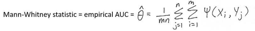
As it turns out, this definition is true because empirical AUC is equal to the Mann-Whitney U-statistic. To quote from DeLong et al.,

When calculated by the trapezoidal rule, the area falling under the points comprising an empirical ROC curve has been shown to be equal to the Mann-Whitney U-statistic for comparing distributions of values from the two samples. […] The Mann-Whitney statistic estimates the probability, theta, that a randomly-selected observation from the population represented by C2 [healthy people] will be less than or equal to a randomly selected observation from the population represented by C1 [sick people].

To phrase the same point yet another way, Wikipedia describes the Mann-Whitney U test as:

a nonparametric test of the null hypothesis that it is equally likely that a randomly selected value from one population will be less than or greater than a randomly selected value from a second population.

Therefore, to summarize,

Note that:

The DeLong Test to Compare AUCs of Two Models

Example Setup

Now that we’ve finished defining the empirical AUC and all the notation, we can move on to a description of how DeLong’s test determines whether one model has a statistically significantly different AUC from an alternative model.

Here is a toy test set of five patients with predictions from two models. We will use this toy test set for the worked example:

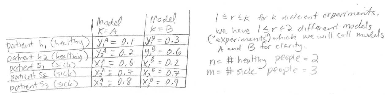
The data set includes two truly healthy patients and three truly sick patients, where their health state was determined in some unambiguous way so that we can consider it “ground truth.” The column for Model A shows predicted disease probabilities for all the patients according to Model A. Following the notation introduced earlier, these predicted probabilities are represented by a Y for the healthy patients and an X for the sick patients. The column for Model B shows the predicted disease probabilities for all the patients according to Model B.

Notice that Model A is a classifier with perfect AUC (which will be explicitly demonstrated later), because all of the healthy patients have lower disease probability than all the sick patients. Model B does not have perfect AUC.

Following the notation of the papers, the total number of models being considered is 1 <= r <= k where k = 2 (because we are only considering 2 models here.) n = 2 (the number of healthy patients) and m = 3 (the number of sick patients.)

Goal of DeLong’s Test

We want to know whether Model A or Model B is better in terms of AUC, where theta-hat(A) is the AUC of Model A, and theta-hat(B) is the AUC of Model B. To answer this question we will calculate a z score:

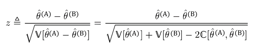
To quote Sun et al.,

Under the null hypothesis, z can be well approximated by the standard normal distribution. Therefore, if the value of z deviates too much from zero, e.g., z > 1.96, it is thus reasonable to consider that [theta(A) > theta(B)] with the significance level p < 0.05.

In other words, if z deviates too much from zero then we can conclude that Model A has a statistically different AUC from Model B with p < 0.05.

To find the z score, we will need to calculate the empirical AUCs, the variance V, and the covariance C. The following sections will show how to calculate these quantities.

(Side Note: the use of “z” here in “z score” is completely unrelated to the use of “z” in the earlier discussion of “z as a decision threshold.”)

Calculating the Empirical AUC for Model A and Model B

 Following the definition of empirical AUC provided earlier, we calculate the empirical AUC for Model A:

Similarly, we calculate the empirical AUC for Model B:

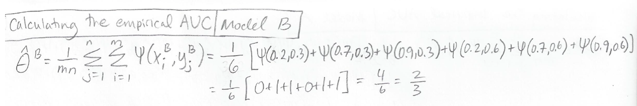
Note that Model A has an AUC of 1.0 because it perfectly ranks all of the diseased patients as having a higher disease probability than all of the healthy patients. Model B has an AUC of 2/3 because it does not perfectly rank all the patients.

Structural Components V10 and V01

The next step needed for DeLong’s test is calculation of V10 and V01, which are referred to as “structural components” by Sun et al.

V10 and V01 will help us find the variance and covariance that we need to calculate the z score. V10 and V01 are defined as follows:

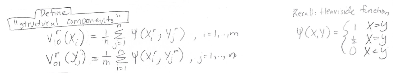
Recall that “r” represents which model we are considering, so we have different structural components calculations for r = A (for Model A) and r = B (for Model B).

For our small example data set, the structural component calculations for Models A and B are as follows:

Matrices S10 and S01

Next, we will use structural components V10 and V01, in combination with our empirical AUCs, to calculate the matrices S10 and S01 which are defined as follows:

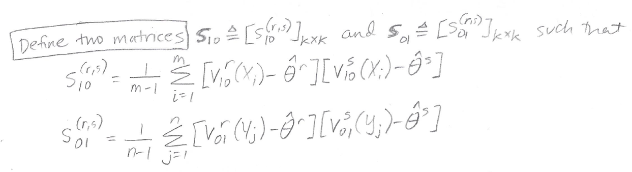
The matrices S10 and S01 are k x k matrices, where k is the total number of models we are considering. Because we are only considering two models (Model A and Model B) each matrix will be 2 x 2.

Here are the calculations for the entries in the matrix S10:

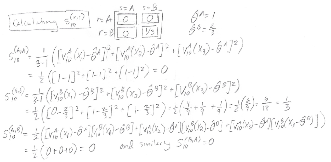
It turns out that for matrix S10, all of the entries are zero except for the (B,B) entry.

Here are the calculations for entries in the matrix S01:

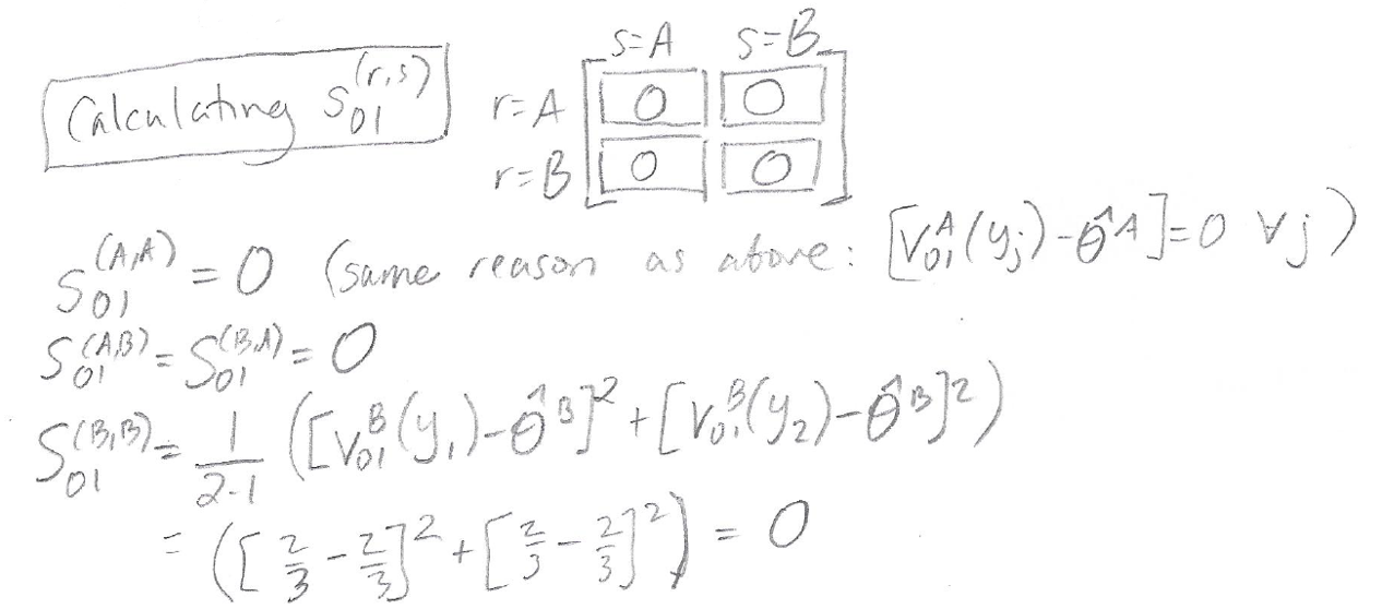
The matrix S01 ends up with all zero entries for this particular example.

Calculating the Variance and Covariance

Now we will use S10 and S01 to obtain a matrix S, where the matrix S contains the variances and covariance that we need in order to get our z score for the DeLong test. All we have to do to get S is sum together S10 and S01, weighted based on 1/ m=3 (the number of sick people) and 1/ n=2 (the number of healthy people) respectively:

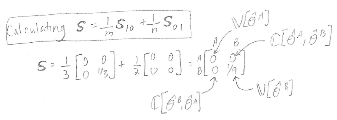
As you can see from the calculation above, our final S matrix contains the variance of the empirical AUC for Model A, the variance of the empirical AUC for Model B, and the covariance of the AUCs for Models A and B. These are key quantities that we need in order to get our z score.

Calculation of the Z Score

To calculate the z score, we plug in the values that we just calculated for the empirical AUCs, variances, and covariance:

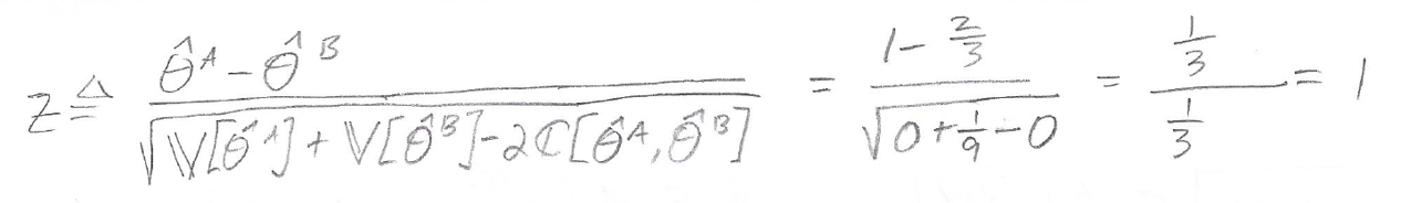
Using the Z Score to Obtain a P-Value

Our calculated z score is 1. How do we obtain a p-value from this?

We are doing a “two-tailed test” because we are trying to claim that the AUC of Model A is different from (“not equal to”) the AUC of Model B.

We can use a lookup table for two-tailed P values for z statistics. In the table, under “tenths” (vertical) we locate 1.0, and under “hundredths” (horizontal) we local 0.00, because our Z-Score is 1.00. The entry in the table at this position is 0.31731, which is our p-value.

Alternatively, to avoid searching through a large table of numbers, we can use an online calculator like this one. We need to select “two-tailed hypothesis” and put in our z score of 1, which produces a p-value of 0.317311 (consistent with the result we got from the lookup table.)

Calculating DeLong’s Test in R

Hand calculations are fine for tiny toy data sets, but for any real data set we will want to use software to compute DeLong’s test. One option is to use the pROC package in R.

Using the pROC package, we first create the two ROC curves to compare, using the roc function. The roc function can be called on a “response” (the ground truth) and “predictor” (the predicted probabilities) as roc(response, predictor).

For our Model A and Model B example, we have:

• response<-c(0,0,1,1,1)
• modela<-c(0.1,0.2,0.6,0.7,0.8)
• modelb<-c(0.3,0.6,0.2,0.7,0.9)
• roca <- roc(response,modela)
• rocb<-roc(response,modelb)

Now that we have built our ROC curves, we can apply the pROC roc.test function to compare the AUCs of two ROC curves.

• roc.test(roca,rocb,method=c(“delong”))

Output:

DeLong’s test for two correlated ROC curves

data: roca and rocb
Z = 1, p-value = 0.3173
alternative hypothesis: true difference in AUC is not equal to 0
sample estimates:
AUC of roc1 AUC of roc2
1.0000000 0.6666667

This matches the result that we obtained manually above.

Another Example of DeLong’s Test in R

Here is another example of DeLong’s test in R, showing how the result is different when different ground truth and predicted probabilities are used:

response<-c(0,0,0,0,0,0,1,1,1,1,1,1,1)
modela<-c(0.1,0.2,0.05,0.3,0.1,0.6,0.6,0.7,0.8,0.99,0.8,0.67,0.5)
modelb<-c(0.3,0.6,0.2,0.1,0.1,0.9,0.23,0.7,0.9,0.4,0.77,0.3,0.89)
roca <- roc(response,modela)
rocb<-roc(response,modelb)

roc.test(roca,rocb,method=c(“delong”))

DeLong’s test for two correlated ROC curves

data: roca and rocb
Z = 1.672, p-value = 0.09453
alternative hypothesis: true difference in AUC is not equal to 0
sample estimates:
AUC of roc1 AUC of roc2
0.9642857 0.7380952

Summary

• DeLong’s test can be used to show that the AUCs of two models are statistically significantly different.
• A ROC curve summarizes sensitivity and (1 – specificity) at different decision thresholds. The AUC is the area under the ROC curve.
• Empirical AUC is calculated using the trapezoid rule on a ROC curve.
• DeLong’s test requires calculation of empirical AUCs, AUC variances, and AUC covariance.
• An R implementation in the pROC package enables quick calculation of DeLong’s test.

About the Featured Image

The featured image is an Egyptian vulture. The original vulture photo was taken by Carlos Delgado CC-BY-SA and is available on Wikipedia here. The photo shown in this post has been modified to include AUC plots and equations related to DeLong’s test. The modified photo is distributed under the same license as the original photo.