Building Custom Image Datasets in PyTorch: Tutorial with Code

In this tutorial, you will learn how to use PyTorch’s inbuilt image data sets, and you will learn how to build your own custom image data sets using any images you want. While this tutorial does focus on image data, the key concepts of customizable datasets in PyTorch apply to any kind of data, including text and structured tabular data.

This tutorial is based on my publicly available repository https://github.com/rachellea/pytorch-computer-vision which contains code for working with custom PyTorch data sets. It also includes code for training and evaluating custom neural networks, overviewed in this post.

By the end of this tutorial, you should be able to:

• Download and use public computer vision data sets with torchvision.datasets (MNIST, CIFAR, ImageNet, etc.);
• Use image data normalization and data augmentation;
• Make your own data sets out of any arbitrary collection of images (or non-image training examples) by subclassing torch.utils.data.Dataset;
• Parallelize data loading with num_workers.

What is a Dataset?

A dataset consists of labeled examples. For image datasets, this means each image is associated with a label. A label could be:

• a vector defining a class like “cat” = [0,1,0] for [dog, cat, bus]
• a vector defining multiple classes like “cat and dog” = [1,1,0] for [dog, cat, bus]
• a matrix defining a segmentation map, where each element of the matrix corresponds to a single pixel of the image and specifies what class that pixel belongs to, e.g. “0” for a pixel that’s part of a dog, “1” for cat, “2” for bus, “3” for chair and so on.

For more information on classification tasks, see this post. For more information on segmentation tasks, see this post.

Downloading Built-In PyTorch Image Datasets

Before building a custom dataset, it is useful to be aware of the built-in PyTorch image datasets. PyTorch provides many built-in/pre-prepared/pre-baked image datasets through torchvision, including:

• MNIST, Fashion-MNIST, KMNIST, EMNIST, QMNIST;
• COCO Captions, COCO Detection;
• LSUN, ImageNet, CIFAR, STL10, SVHN, PhotoTour, SBU, Flickr, VOC, Cityscapes, SBD, USPS, Kinetics-400, HMDB51, UCF101, and CelebA.

After torchvision is imported, the provided datasets can be downloaded with a single line of code. Here is an example of downloading the MNIST dataset, which consists of 60,000 train and 10,000 test images of handwritten digits. Each image is grayscale and 28 x 28 pixels:

import torchvision
mnist = torchvision.datasets.MNIST('path/to/mnist_root/',download=True)

In the above code snippet, you would replace ‘path/to/mnist_root/’ with the absolute path to the directory in which you would like to save the MNIST images.

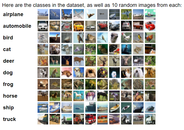
Here’s an example of how to download the CIFAR-10 dataset:

cifar10 = torchvision.datasets.CIFAR10('path/to/cifar10_root/',download=True)

CIFAR-10 includes 50,000 train and 10,000 test images. They are all natural images, in color, 32 x 32 pixels in size.

You can specify a particular subset of a downloaded dataset (e.g. train, val, or test). The syntax is simple and varies only a little depending on the dataset you are using. The necessary arguments to specify a particular subset of a downloaded dataset are all documented here, on the torchvision datasets page, for each dataset separately.

As an example, to specify the train or test set of MNIST, an argument called “train” is provided which can be set to True or False:

To specify the training set of MNIST, set train=True.

mnist_train = torchvision.datasets.MNIST('path/to/mnist_root/', train=True)

To specify the test set of MNIST, set train=False.

mnist_test = torchvision.datasets.MNIST('path/to/mnist_root/', train=False)

To specify the train or val set of the VOC 2012 segmentation dataset, an argument called “image_set” is provided, which can be set to “train” or “val”:

vocseg_train = torchvision.datasets.VOCSegmentation('path/to/voc_root/', year='2012',image_set='train')

vocseg_val = torchvision.datasets.VOCSegmentation('path/to/voc_root/',year='2012',image_set='val')

Avoiding Excessive Downloads

For some of the built-in PyTorch datasets, the initial download can take a significant amount of time, depending on dataset size and your Internet speed. Thankfully, if you have already downloaded the dataset once, you don’t need to download it again on that machine as long as you specify the directory in which you originally downloaded the dataset. For example, if you’ve already downloaded MNIST to the directory ‘path/to/mnist_root/’, then you can access the dataset without downloading it again as long as the path you provide is ‘path/to/mnist_root/’. You can also explicitly specify NOT to download the dataset again by setting download=False, which means you will get an error if for some reason the path you provided is incorrect.

#The first time we use this training set, we download it to a particular location
mnist_train = torchvision.datasets.MNIST('path/to/mnist_root/', train=True)

#The second time we use this training set, we don't need to download it and we can just load it from the location we specified before:
mnist_train = torchvision.datasets.MNIST('path/to/mnist_root/', train=True, download=False)

Using Built-In PyTorch Image Datasets with the DataLoader Class

To actually use a dataset, we need to be able to pick out examples from that dataset and create batches of them to feed to our model. The PyTorch DataLoader takes in a dataset and makes batches out of it. It’s nice that DataLoader takes care of batching, because it means we don’t need to write any tedious code to select out random subsets of our dataset.

Here is an example of how to create a training data loader for MNIST using the provided DataLoader class:

import torch
import torchvision

mnist_train = torchvision.datasets.MNIST('path/to/mnist_root/',train=True)
train_data_loader = torch.utils.data.DataLoader(mnist_train,
                                          batch_size=32,
                                          shuffle=True,
                                          num_workers=16)
for batch_idx, batch in enumerate(train_data_loader):
    #inside this loop we can do stuff with a batch, like use it to train a model

Here is an example of how to create a test data loader for MNIST:

mnist_test = torchvision.datasets.MNIST('path/to/mnist_root/',train=False)
test_data_loader = torch.utils.data.DataLoader(mnist_test,
                                          batch_size=32,
                                          shuffle=False,
                                          num_workers=16)
for batch_idx, batch in enumerate(test_data_loader):
    #do stuff

Normalizing Data for Neural Network Models

Before providing image data to a neural network, the images must be normalized so that numerically the input data is roughly in the range [0,1] or [-1,1]. Neural networks have more stable training when the magnitude of the data on which they are trained is in approximately this range. It’s extremely unlikely that you would be able to successfully train a neural network model on images with raw RGB pixel values which are in the range 0 to 255.

PyTorch provides multiple options for normalizing data. One option is torchvision.transforms.Normalize:

You can see that the above Normalize function requires a “mean” input and a “std” input. The “mean” should be the mean value of the raw pixels in your training set, for each color channel separately. The “std” should be the standard deviation of the raw pixels in your training set, for each color channel separately. If you have a big data set you will want to compute these values once and then store them, rather than re-calculate them every time. Note that you must only use the training set to calculate the mean and standard deviation because if you use the whole data set, you will be leaking information about your test set into your training process by including it in the mean/std calculation.

Preprocessing Data for Models Pre-Trained on ImageNet

PyTorch provides models pre-trained on ImageNet. When preparing data to feed to these models, we must consider that all these models expect their input images to be preprocessed in a particular way. The images must be 3-channel and RGB, with shape (3 x H x W) where H and W are expected to be at least 224. Furthermore, the pixel values must be within the range [0, 1] and should be normalized using mean = [0.485, 0.456, 0.406] and std = [0.229, 0.224, 0.225]. These mean and std values were calculated on ImageNet using the process described in the previous section. The following transform will normalize using these ImageNet specifications:

normalize = transforms.Normalize(mean=[0.485, 0.456, 0.406],
                                 std=[0.229, 0.224, 0.225])

Data Augmentation

Data augmentation allows you to encourage a model’s predictions to be invariant to certain kinds of changes, such as flips or rotations for images. PyTorch provides many transforms for image data augmentation in torchvision.transforms including color jitter, grayscale, random affine transformations, random crops, random flips, random rotations, and random erasing. It is possible to aggregate multiple transformations with torchvision.transforms.Compose(transforms).

Note that if you are doing an object detection or segmentation task where the ground truth is “image-like” and the same shape as the input image, you need to apply equivalent data transformations to the ground truth and the input image. For example, if you apply a horizontal flip to an input image, you also need to horizontally flip a segmentation ground truth for that image.

Here are some examples of data transformations for data augmentation, using a public domain dog picture from Wikipedia:

Making Your Own Datasets: Overview

You can make a PyTorch dataset for any collection of images that you want, e.g. medical data, random images you pulled off the Internet, or photos you took. Examples of various machine learning data sets can be found here.

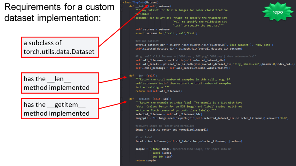
The requirements for a custom dataset implementation in PyTorch are as follows:

• Must be a subclass of torch.utils.data.Dataset
• Must have __getitem__ method implemented
• Must have __len__ method implemented

After it’s implemented, the custom dataset can then be passed to a torch.utils.data.DataLoader which can then load multiple batches in parallel. This is really nice – it means that all you have to do is define where to find your image data and how to prepare it (i.e., define a dataset), and then PyTorch takes care of all the batching and parallel data loading so you don’t have to!

Making Your Own Datasets: TinyData Example

The repository for this tutorial includes TinyData, an example of a custom PyTorch dataset made from a bunch of tiny multicolored images that I drew in Microsoft Paint. Here’s a picture showing what the images in the data set look like:

Here’s a screenshot of the CSV (displayed in Excel) that defines what the labels are for each image:

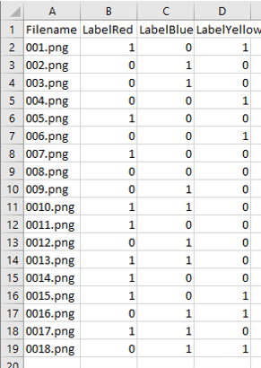
As you can see from the above, TinyData is a dataset for a multilabel classification task, in which each image is associated with one or more of the label categories – red, blue, or yellow, for whether or not that particular color appears within the image.

Code for TinyData PyTorch Dataset

Now let’s take a look at the code that defines the TinyData PyTorch dataset.

This code can be found within the load_dataset directory of the repository. It’s split into two modules, custom_tiny.py which defines the TinyData dataset, and utils.py which defines image preprocessing functions.

At a high level, if we look in custom_tiny.py at the TinyData class, we can see that TinyData meets the 3 requirements listed above for implementation of a custom dataset in PyTorch:

Let’s now consider each of these required pieces:

A subclass of torch.utils.data.Dataset: all we need to do in order to make our dataset a subclass of the PyTorch Dataset is put torch.utils.data.Dataset in parentheses after the name of our class, like MyClassName(torch.utils.data.Dataset) if we’ve only imported torch, or MyClassName(Dataset) if we’ve used a more specific import, “from torch.utils.data import Dataset.” Making our dataset a subclass of the PyTorch Dataset means our custom dataset inherits all the functionality of a PyTorch Dataset, including the ability to make batches and do parallel data loading.

__len__ method: this method simply returns the total number of images in the dataset. You can see in the code for TinyDataset that we define self.all_filenames to contain all the names of the image files in our data directory, so then we can implement the __len__ method as simply len(self.all_filenames). It’s not a good idea to hard-code the number of images in your data set; it’s better to calculate the number of images based on the contents of the directory in which the images are stored.

__getitem__ method: this method must take in an integer value “idx”. The method then uses that integer value to select a single example from the dataset, e.g. by indexing into a list of file names. Finally, the method returns the example so that it can be provided to a model. The example, at a minimum, needs to include an image and its corresponding label. The image should already be fully processed so that it can be fed directly into the model – all normalization and data augmentation steps should be applied to the image before this method returns it.

You can see in the example code for TinyData that its __getitem__ method includes a few steps:
(1) selecting the file located at the index “idx”, via selected_filename=self.all_filenames[idx];
(2) loading the image stored at this location, using the PIL library;
(3) applying data processing steps, in this case implemented by the function to_tensor_and_normalize() which is defined in the utils module;
(4) loading the label for this image;
(5) creating an example (called “sample”) by defining a Python dictionary that contains the image data, the label, and also the integer index. You technically don’t need to provide the integer index but it can be helpful for learning purposes so it’s included here.

Keep Data Processing Code Separate

It’s good practice to keep the code that does data processing steps in a separate module from your dataset definition. Why?

Reason #1: If you’re going to run a lot of different kinds of experiments, chances are your image processing code will grow over time, and you don’t want to clutter up the module that defines your dataset with a bunch of data processing functions. The data processing code in this tutorial is extremely simple – only a few lines long – but on principle I’ve put it into its own module, utils.py. (Really, it’s a good idea to have a more specific module name than “utils” but for this tutorial it suffices.)

Reason #2: You may want multiple different datasets to use the same data processing steps. If all the data processing functions are defined in some “processing module”, then each dataset module can import from this single “processing module” and the code stays organized. As an example of this, utils.py is imported and used by both custom_tiny.py (defining our tiny custom dataset) as well as by custom_pascal.py (which defines a PASCAL VOC 2012-based dataset, discussed later in this post).

If we were doing a lot of customized data augmentation, the functions for doing that would be defined in utils.py too.

Defining Train vs Validation vs Test Data

You don’t need to define separate Dataset classes for train, validation, and test data. In fact, doing so would be undesirable, since it would require your codebase to contain a lot of redundant code. Instead, to enable a single Dataset class to be used for training, validation, or test data, you can use an argument to determines where your Dataset will go looking for images. In the TinyData example, this argument is called “setname” and it determines the directory from which the TinyData class will load images.

Training Models on TinyData

To train neural networks on the TinyData, you can run these commands:

python Demo-1-TinyConvWithoutSequential-TinyData.py
python Demo-2-TinyConv-TinyData.py

You don’t need a GPU to run the above commands because the data set is so tiny.

Custom Dataset for PASCAL VOC 2012

As we’ve seen from the TinyData example, PyTorch datasets certainly come in handy when you want to use your own images. It turns out that PyTorch datasets also come in handy if you want to use existing PyTorch datasets in a different way than the default. Let’s take a look at load_dataset/custom_pascal.py (also in the tutorial repository) to understand why and how this is done.

custom_pascal.py defines a dataset for the PASCAL VOC 2012 dataset. PASCAL is a data set of natural images labeled with segmentation maps for the following classes: ‘airplane’, ‘bicycle’, ‘bird’, ‘boat’, ‘bottle’, ‘bus’, ‘car’, ‘cat’, ‘chair’, ‘cow’, ‘dining_table’, ‘dog’, ‘horse’, ‘motorbike’, ‘person’, ‘potted_plant’, ‘sheep’, ‘sofa’, ‘train’, and ‘tv_monitor’. Each image may have more than one class.

It turns out that PyTorch provides a class for loading PASCAL already. Here’s an example of using the built-in PyTorch class to load the PASCAL VOC 2012 training set:

pascal_train = torchvision.datasets.VOCSegmentation(voc_dataset_dir, year='2012',image_set='train',download=False)

If PyTorch already has a built-in class for PASCAL, called VOCSegmentation, why did we bother defining a custom class for PASCAL in custom_pascal.py? There are two main reasons:

(1) So we can combine the PASCAL dataset with SBD and create a larger overall dataset;

(2) So we can use classification labels instead of segmentation labels.

Combining Two Datasets: PASCAL + SBD

The PASCAL dataset in research papers is often combined with the SBD dataset. In order to train a single model on both the PASCAL and SBD datasets we need to “mix together” these datasets somehow. The least ugly way to do this is to load both PASCAL and SBD together within a custom dataset class, which we do within our custom class:

#Define dataset
if setname == 'train':
    #In the training set, combine PASCAL VOC 2012 with SBD
    self.dataset = [torchvision.datasets.VOCSegmentation(voc_dataset_dir, year='2012',image_set='train',download=False),
                    #SBD image set train_noval excludes VOC 2012 val images
                    torchvision.datasets.SBDataset(sbd_dataset_dir, image_set='train_noval', mode='segmentation',download=False)]

elif setname == 'val':
    self.dataset = [torchvision.datasets.VOCSegmentation(voc_dataset_dir, year='2012',image_set='val',download=False)]

Then at the beginning of our __getitem__ method, we simply check to see whether we need to select our image from the PASCAL dataset or the SBD dataset, depending on how big the integer idx is:

if idx < len(self.dataset[0]):
    chosen_dataset = self.dataset[0]
else:
    chosen_dataset = self.dataset[1]
    idx = idx - len(self.dataset[0])

The last consideration is defining our __len__ method appropriately so that we taken into account the sizes of both datasets:

def __len__(self):
    if self.setname == 'train':
        return len(self.dataset[0])+len(self.dataset[1])
    elif self.setname == 'val':
        return len(self.dataset[0])

Because the __len__ method correctly reflects the combined size of PASCAL and SBD, the random integer idx that PyTorch produces when it’s sampling from our dataset will sometimes cause the __getitem__ function to return a PASCAL image, and other times it’ll cause __getitem__ to return an SBD image.

Changing a Dataset’s Labels: Segmentation -> Classification

The second reason we’ve defined a custom dataset for PASCAL is to use different labels. The PASCAL dataset as defined by PyTorch is set up to enable training segmentation models. Thus, the ground truth for each image is a segmentation map.

But what if instead of training a fully supervised segmentation model, we want to train a classification model, or a weakly supervised segmentation model that relies only on classification labels? In that case we need labels in a different format, namely a multi-hot vector indicating presence or absence of each class.

We can define this new kind of label within our custom dataset class. That is done in the custom_pascal.py function get_label_vector(), which takes in the default segmentation map label and transforms it into a multi-hot presence/absence vector. Then, __getitem__ makes use of get_label_vector() to transform the segmentation map label into the classification label that we want to use.

The module custom_pascal.py also contains additional useful code, including functions to visualize the images in the dataset and visualize the ground truth segmentation maps. It also includes the mapping from the integer class labels to their corresponding descriptive names like “cat” or “bus”.

Training Models on the Custom PASCAL VOC 2012 Dataset

To train neural networks on the custom PASCAL VOC 2012 dataset (which includes SBD), you can run these commands, ideally on a machine with a GPU:

python Demo-3-VGG16-PASCAL.py
python Demo-4-VGG16Customizable-PASCAL.py 

Unit Tests

It’s always a good policy to write unit tests for your data processing. If you process your data incorrectly, then any models you train on it will be wrong.

An example of unit testing can be seen in src/unit_tests.py. To run the unit tests, you can use this command:

python Demo-0-Unit-Tests-and-Visualization.py

The above command will also run the PASCAL VOC 2012 dataset visualization.

(Side note on code organization: If you’re writing a lot of unit tests they should all really go in their own tests directory that’s at the same level as src. Then each module in src can have a corresponding unit testing module within tests.)

Custom Medical Dataset

The public GitHub repository rachellea/ct-net-models includes code defining a PyTorch dataset for CT volume data, including extensive data preprocessing steps and data augmentation.

Parallel Data Loading with num_workers

I’ve mentioned that PyTorch takes care of loading multiple batches in parallel. You can control how many batches are loaded in parallel by defining num_workers in your DataLoader:

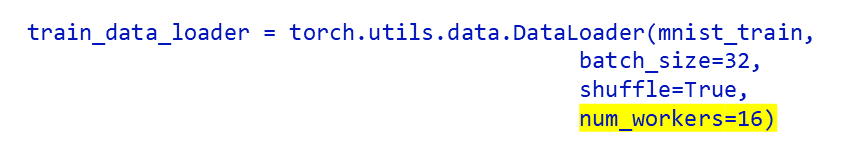
num_workers determines the number of processes that will be used to load your data. Each process will load one batch.

If you want to do single-process data loading, and only load one batch at a time, then you set num_workers = 0. Because this will cause PyTorch to launch only one data loading process, it may be slower overall, and your GPU may have a lot of idle time as it waits for the CPU to finish processing the next batch. One great reason to set num_workers = 0 is if you’re using a Windows machine and want to use the Python debugger. Because of how Windows deals with multiprocessing, you need to set num_workers = 0 in order to use the Python debugger with PyTorch on Windows. However, once your program is debugged, you can then increase num_workers and run the code without the debugger.

If you want to do multi-process data loading, then you need to set num_workers to a positive integer specifying the number of loader worker processes. In this setting, while the GPU computes on one batch, other batches are being loaded. For example, if you choose num_workers=16, then there will be 16 processes loading your batches, which means roughly speaking you’ll be loading 16 batches at the same time. If you choose num_workers well, then the GPU won’t have to wait at all between batches – as soon as it’s done using one batch, the next is already ready to go.

You need to choose num_workers carefully, otherwise you could overload your machine by trying to load too many batches at the same time. This is particularly relevant if you are working with massive images like CT volumes or if you are doing heavy amounts of data preprocessing.

There are no strict rules about how to choose num_workers. Here are some general tips that may be useful:

• Keep in mind that higher is not always better. You will choke your machine if you make num_workers too high, causing slowness or memory errors.
• A decent rule of thumb is to use num_workers equal to the number of CPU cores you have available.
• If you need to maximally optimize performance, just do experiments with different values of num_workers, time how long an epoch takes, and then choose the value that leads to the fastest time. This isn’t a terribly “mentally satisfying” approach (because it feels like you should be able to calculate the optimal number of workers easily) but this experimental measurement is the quickest and most reliable way to figure out a good num_workers to use.
• Remember that you will likely want to lower num_workers if you suddenly switch from training one model at a time to training multiple models at a time.

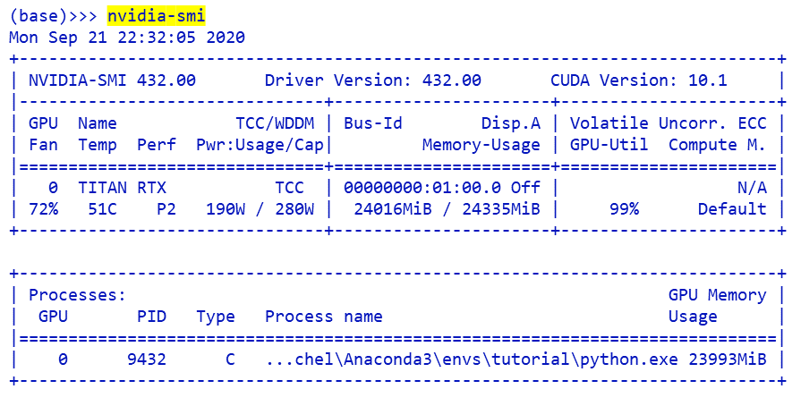
If you are using an NVIDIA GPU you can check memory usage with nvidia-smi:

Miscellaneous Tips

• If you have a training loop that iterates over epochs, make sure you put the data loader outside of the epoch loop. Otherwise you will initialize your data loader once every epoch which is (a) unnecessary and (b) eats up your memory usage.
• If you are using Git for version control, store image datasets outside of your Git repository. The only reason that “tiny data” is in the tutorial repo is because this is a tutorial and the data is unrealistically small.
• Similar to the preceding bullet, it’s also a good idea to store results files outside of your Git repository, as results for image models frequently contain large files (e.g. visualizations).

Summary

• PyTorch’s torchvision library includes numerous built-in datasets including MNIST and ImageNet.
• PyTorch’s DataLoader takes in a dataset and makes batches out of it.
• torchvision.transforms can be used to normalize data and/or perform data augmentation.
• Custom datasets in PyTorch must be subclasses of torch.utils.data.Dataset, and must have __getitem__and __len__ methods implemented. Beyond that, the details are up to you!
• Custom datasets in PyTorch can also make use of built-in datasets, to combine them into one bigger dataset and/or compute different labels for each image.
• Setting the num_workers DataLoader argument to some positive integer value n means that n processes will load batches in parallel.

Happy dataset creation!

About the Featured Image

The featured image makes use of a neural network visualization from Wikipedia (Creative Commons license).