

If you are interested in creating your own medical image data set for a machine learning project, this post is for you. You may also be interested in this post if you work with publicly-available medical imaging datasets and would like some further insight into how these datasets are created.
In this post, you will learn:
- The basics of DICOM, the file format in which medical images are stored in health systems;
- How to use Python to bulk download tens of thousands of medical images as DICOMs from health system storage;
- How to clean the DICOMs and convert them into numpy arrays using an end-to-end Python pipeline that I developed while preparing the RAD-ChestCT data set of 36,316 chest computed tomography volumes, one of the largest volumetric medical imaging datasets in the world.
This post is based in part on an appendix to my recent paper, “Machine-Learning-Based Multiple Abnormality Prediction with Large-Scale Chest Computed Tomography Volumes” (published in the journal Medical Image Analysis and also available on arXiv). If you find this post helpful in your own research, please consider citing our paper. The code for this post is publicly available on GitHub: rachellea/ct-volume-preprocessing.
There are many different kinds of medical images including projectional x-rays, computed tomography (CT), magnetic resonance imaging (MRI), and ultrasound. Throughout this post, I will be using CT scans as a running example, although a lot of the concepts discussed in this post are relevant to other kinds of medical images.
Choosing Scans to Download
The first step in building a medical image data set is choosing what scans to download. One way to choose scans is by making use of databases of radiology reports.
Every time a medical image is acquired, a radiologist writes a report describing the abnormalities that are present or absent in the medical image, to help other doctors who are not medical imaging experts understand what aspects of that image are most important for patient care. These written reports are stored in health system databases. A table of radiology reports will often include the report text itself, as well as three important identifying fields: the patient’s medical record number (MRN), the accession number, and the protocol description.
A medical record number (MRN) uniquely identifies a patient within a health system. The MRN is critical for defining a train/validation/test split in which no patient appears in more than one set. Images from the same patient must all be grouped into the same set because even if the scans occurred years apart, they are correlated because they depict the same individual.
The accession number uniquely identifies the medical imaging event. It is an alphanumeric identifier, e.g. “AA12345” (different from the MRN) that specifies a particular occurrence of a particular patient getting imaged. The accession number of a medical imaging event is used for both the written report and the image files associated with that event, which enables matching up written reports with their corresponding images.
Finally, the protocol description is a string that describes what kind of medical imaging was performed. A protocol can be thought of as a “recipe” for obtaining a certain kind of medical image. The “protocol description” is the title of the recipe. The protocol description typically specifies the modality (e.g. CT vs. MRI vs. ultrasound), the part of the body that was imaged, and other details about how the imaging was acquired (e.g. whether contrast was used).
Here are some example protocol descriptions for CT scans:
- CT abdomen pelvis with contrast
- CT chest wo contrast w 3D MIPS Protocol
- CT chest abdomen pelvis with contrast w MIPS
- CT ABDOMEN PELVIS W CONT
- CT abdomen pelvis without contrast
- CT brain without contrast
- CT chest PE protocol incl CT angiogram chest w wo contrast
- CT CHEST W/ENHANCE
- CT CHEST
- CT MIPS
Filtering Scans by Protocol
One critical component of a protocol description is the specification of what part of the body was imaged. Different anatomic locations for imaging include chest only, abdomen only, pelvis only, chest/abdomen/pelvis together, head, spine, arm, hand, and more.
Some examples of CTs of different anatomic regions are shown here:
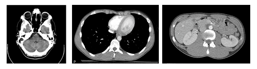
Examples of CT scans of different anatomical regions. From left to right, the images show the head, the chest, and the abdomen. The images are from Wikipedia (Creative Common licenses): head CT, chest/abdomen CT.
When building a medical imaging data set, it is important to consider whether it is necessary to combine images from different body regions or whether it makes the most sense to focus on only one body region. The DeepLesion data set includes many different body regions because the goal is to build models to identify “lesions” which is defined broadly as any focal abnormality at all. In contrast, the MIMIC-CXR data set includes only images of the chest because the focus is on specifically chest abnormalities. In general, you should have a very good reason for combining images from different body regions in the same data set, because unfiltered images of different body regions will show mutually exclusive pathology – for example, a head CT scan will never show pneumonia since pneumonia is specific to the lungs, while a chest CT scan will never show a stroke since strokes are specific to the brain.
The chest is a popular body region for medical imaging datasets, because it includes multiple major organs (most notably the heart and lungs), and can display a diverse array of pathological findings including lung nodules, interstitial lung disease, pleural effusions, lung cancer, infections, inflammation, and edema (Purysko 2016). Medical imaging data sets focused on the chest include MIMIC-CXR, CheXpert, and RAD-ChestCT.
A second important component of a protocol is the description of whether contrast was used, and how. Contrast is a radiopaque liquid, paste, or tablet made from barium, iodine, or gadolinium that is swallowed, injected into arteries, injected into veins, or delivered by enema in order to highlight particular anatomical structures (Lusic 2013). Different kinds of contrast will look different. On a CT scan, contrast appears bright white. The type of contrast agent, the method of administration, and the timing relative to the acquisition of the scan can all be specified in the protocol description.
A CT pulmonary angiogram is a type of chest CT in which contrast is injected to fill the pulmonary blood vessels; it is often used for the diagnosis of pulmonary embolism, which is a clot in the pulmonary blood vessels. The clot appears greyer than the surrounding white contrast and is thus easier for the radiologist to identify (Wittram 2004).
Contrast CTs of the abdomen and pelvis can be obtained to evaluate for appendicitis, diverticulitis, and pancreatitis (Rawson 2013).
In other cases, contrast is unnecessary, or even contraindicated — for example if the patient has kidney disease, is pregnant, or has previously had an allergic reaction to contrast agents.
The RAD-ChestCT data set includes only chest CT scans obtained without intravenous contrast. To select accessions numbers for the RAD-ChestCT data set, I filtered the table of radiology reports to choose only scans with a lowercased protocol description matching either “ct chest wo contrast w 3d mips protocol” (the second most common protocol overall) or “ct chest without contrast with 3d mips protocol.” This yielded 36,861 CT reports, with accession numbers that I could then use to download the actual CT images associated with each report.
The Data Interchange Standard for Biomedical Imaging (DICOM)
Before getting in to the details of downloading and processing the images, it’s important to introduce DICOM.
The Data Interchange Standard for Biomedical Imaging (DICOM) is the standard format in which medical images are stored in a health system. An image in DICOM format is saved as a pixel array with associated metadata. The metadata includes information about the patient, including the patient’s name and birthday. The metadata also includes information about the image itself, such as the name of the device used to acquire the image and certain imaging parameters. While several DICOM attributes in the metadata should always be available (e.g. the patient’s name), other DICOM attributes are unique to a particular scanner or machine, or unique to a particular kind of imaging, and thus may not be available for all DICOM files. This means that the exact set of attributes available in a particular DICOM file is not guaranteed to be the same as the attributes in another DICOM file.
For the purposes of creating the RAD-ChestCT dataset, several DICOM attributes were particularly important. These attributes are summarized in the following table which includes excerpts from the DICOM Standard Browser by Innolitics:

DICOM attributes useful for cleaning CT volumes. Source: the Innolitics DICOM browser: Image Type, Image Orientation (Patient), Image Position (Patient), Rescale Intercept, Rescale Slope, Pixel Spacing, Gantry/Detector Tilt.
Downloading Medical Images
Medical images can be downloaded one-by-one using many software programs available in health systems. However, individual download is not practical for creation of a large medical imaging data set. Automated mechanisms are required in order to collect a large number of images.
In a health system, medical images often live in a Vendor Neutral Archive, or VNA. To quote Wikipedia, “a Vendor Neutral Archive (VNA) is a medical imaging technology in which images and documents […] are stored (archived) in a standard format with a standard interface, such that they can be accessed in a vendor-neutral manner by other systems.” Thus, a VNA is basically a place in a health system where a whole bunch of medical images in DICOM format are stored so that they can be easily accessed by various devices throughout the hospital system.
To create RAD-ChestCT, I queried all 36,861 selected chest CT scan accession numbers using an application programming interface (API) developed for Duke’s vendor neural archive. The code is available here; note that the required passkeys have all been taken out for security reasons.
Because I was downloading a lot of CT scans, the download process required 49 days. Overall, the download had a 99% success rate, with 36,316 volumes acquired out of 36,861 initially specified.
One important consideration for bulk downloading CT scans based on an accession number is how to select the series.
Selecting the Series
A single CT scanning event is indicated by one unique accession number, but that accession number might correspond to more than one CT volume. For example, if the first scan is of insufficient quality, a second scan may be obtained. Additionally, once the scanning is finished, the radiologists who interpret the scans may create “reformats” which are alternative representations of the scan data that display the patient’s body in a different way.
Each separate CT scan obtained during the CT scanning event and each separate reformat created afterwards is referred to as a separate “series.”
When downloading tens of thousands of scans, each with multiple series, it is impractical to assume that the “best and most representative series” could be hand-picked for each scan. Instead, an automated process is needed to choose the series.
For RAD-ChestCT, I defined the following process for selecting the series automatically:
First, I made use of the ImageType DICOM attribute to only consider scans marked as ORIGINAL. I excluded scans marked as DERIVED, SECONDARY, or REFORMATTED.
Next, for accession numbers with more than one ORIGINAL series, I selected the series with the greatest number of slices.
CT scans are volumetric, represented as a stack of 2D images (“slices”). An ORIGINAL CT series will consist of axial slices that are not cropped, e.g.:
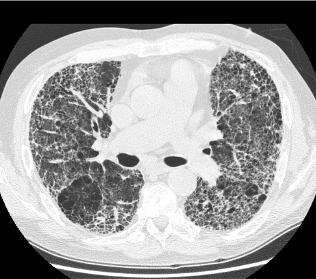
A CT scan slice in the layout expected of ORIGINAL CT series. This CT slice shows extensive pulmonary fibrosis. It is from Wikipedia and released under a Creative Commons license.
Here are a couple examples of non-ORIGINAL CT series:
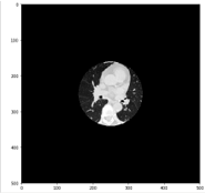
A non-original CT series. In this non-original series, most of the other anatomy has been cropped out to focus on the heart. Image by author.

A non-original CT series. In this non-original series, two sagittal view of the patient have been stacked on top of each other. Image by author.
Code
The code for downloading original CT volumes in bulk, selecting the ORIGINAL series, and logging information about the download progress is publicly available on GitHub here: rachellea/ct-volume-preprocessing/download_volumes.py.
CT Volume Preprocessing: DICOM to numpy
Unfortunately, raw DICOMs cannot be used as the input to any major machine learning framework. The DICOMs must first be processed before they can be computationally analyzed. I developed an end-to-end Python pipeline that will process separate DICOM files corresponding to different slices of one CT scan into a single 3D numpy array compatible with PyTorch, Tensorflow, or Keras.
Here’s a quick summary of the processing steps required, with more details provided in the subsequent sections:
- Stack up the CT slices in the right order;
- Double check that the CT scan is in the desired orientation;
- Convert the pixel values to Hounsfield Units (HU) using the DICOM attributes RescaleSlope and RescaleIntercept;
- Clip the pixel values to [-1000 HU,+1000 HU], the practical lower and upper limits of the HU scale, corresponding to the radiodensities of air and bone respectively;
- Use SimpleITK to resample each volume to 0.8 x 0.8 x 0.8 mm to enable a consistent physical distance meaning of one pixel across all patients;
- Convert the pixel values to 16-bit integers and save with lossless zip compression to reduce storage requirements.
Ordering Slices
Separate DICOM files are saved for each axial slice of a CT volume. Relative to a standing person, an “axial slice'” represents a horizontal plane through the body (the same plane formed by a belt around the waist):

Anatomical planes. The axial plane is shown in green. A CT scan is typically saved as a stack of 2D images in the axial plane, with a separate DICOM file for each 2D image. This image has been modified from this Wikipedia image by David Richfield and Mikael Haggstrom and is available under the Creative Commons license.
The separate axial slices must be stacked in the correct order in order to recreate the 3D volume — a process which is surprisingly nontrivial, but critical in order to obtain usable data. If slices are put together in the wrong order, the volumetric representation is destroyed.
The most intuitive DICOM attribute to use for slice ordering is called InstanceNumber. This attribute is supposed to specify the order of the slices using integers. Unfortunately, this attribute is not reliable and is filled incorrectly by some CT scanners, so InstanceNumber should never be used for slice ordering.
The most reliable way to order slices is to make use of the ImageOrientationPatient and ImagePositionPatient attributes.
There are 12 possible orientations of a patient within a CT volume:
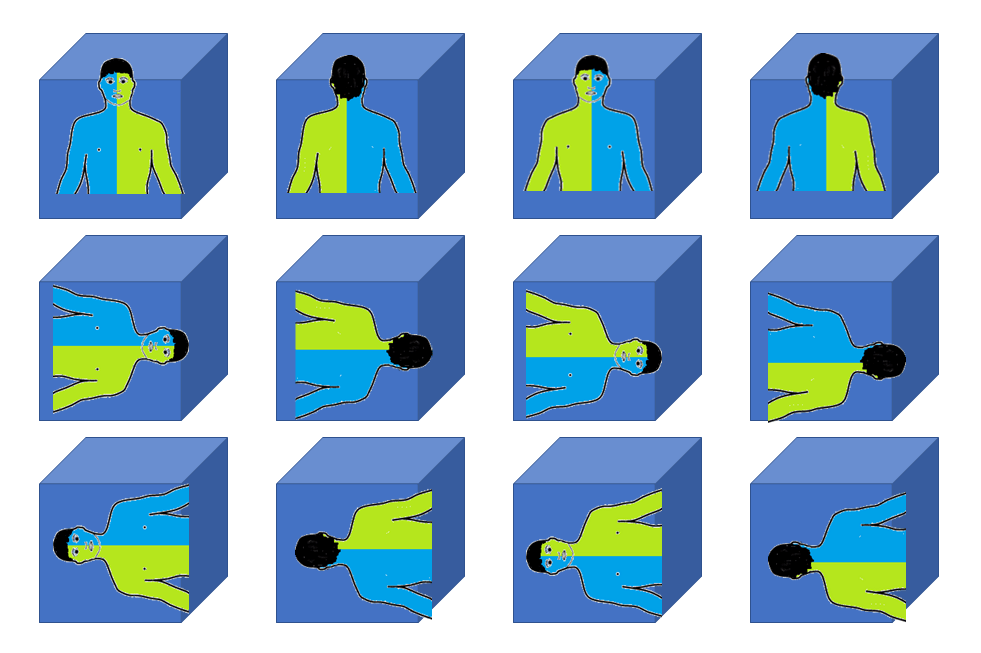
The 12 possible orientations of a person within a volume. Orientation is important because humans are asymmetrical on the inside (e.g. the heart is towards the left, the stomach is on the left, the liver is on the right). Image by Author. Human silhouette modified from Wikipedia human body schemes (Creative Commons License).
In a DICOM file, the attribute ImageOrientationPatient specifies the patient’s orientation and is needed in order to determine which direction is the “z-direction” (the head-to-toe or craniocaudal direction along which axial slices are stacked). Typically, patients are presented in the “1,0,0,0,1,0” orientation for a chest CT, but the orientation is still important to verify as it can sometimes vary.
Given the patient orientation it is possible to determine which value stored in the ImagePositionPatient attribute is the z-position. The z-position reflects a physical distance measurement of the craniocaudal (head-to-toe) location of the slice in space. By sorting slices according to their z-position, it is possible to obtain the correct slice ordering and reconstruct the full 3D volume.
Here’s an excerpt from the sorted z-positions for the slices of one CT scan (the full list of sorted z-positions is much longer, since there are 512 slices):
[-16.0, -16.6, -17.2, -17.8, -18.4, -19.0, -19.6, -20.2, -20.8, -21.4, -22.0, -22.6, -23.2, -23.8, -24.4, -25.0, -25.6, -26.2, -26.8, -27.4, -28.0, -28.6, -29.2, -29.8, -30.4, -31.0, -31.6, -32.2, -32.8, -33.4, -34.0, -34.6, -35.2, -35.8, -36.4, -37.0, -37.6, -38.2, -38.8, -39.4, -40.0, -40.6, -41.2, -41.8, ..., -318.4, -319.0, -319.6, -320.2, -320.8, -321.4, -322.0, -322.6, -323.2, -323.8, -324.4, -325.0, -325.6, -326.2]In my pipeline, I made use of combine_slices.py from Innolitics to perform the slice ordering step based on the DICOM attributes ImageOrientationPatient and ImagePositionPatient.
Rescaling Pixel Values to Hounsfield Units
A CT scanner’s measurements are represented with Hounsfield Units.
Hounsfield Units indicate the radiodensity of a material, and range from approximately -1000 HU (air) to +1000 HU (bone), with water in the middle at 0 HU. In some cases, HU can reach around +2000 for very dense bone (e.g. the cochlea in the ear), but most tissues are in the range -600 to +100 HU (Lamba 2014).

The Hounsfield scale. Image by Author.
Raw pixel values in DICOMs have undergone a linear transformation out of Hounsfield Units to enable efficient disk storage. This transformation must be reversed to obtain pixel values in Hounsfield units (HU) once again. The DICOM standard includes the attributes RescaleSlope and RescaleIntercept which are the m and the b in the equation y = mx + b, needed to linearly transform the raw pixel values x stored in the DICOM pixel array into Hounsfield units y. All raw pixel values from the DICOM must be rescaled to HU using the RescaleSlope and RescaleIntercept attributes. This ensures that a particular numerical value for a pixel indicates the same radiodensity across all scans. Note that RescaleSlope is usually equal to 1 and RescaleIntercept is usually equal to -1024 but it is always a good idea to double check.
After converting to HU, the pixel values can be clipped to [-1000 HU,+1000 HU], which represent practical lower and upper limits of the HU scale, corresponding to the radiodensities of air and bone respectively.
Resampling
In addition to ensuring that the pixel values have consistent radiodensity meaning across the whole data set by converting to Hounsfield units, it is also important to ensure that each pixel represents a consistent volume throughout the whole data set. A DICOM header includes the attribute PixelSpacing which includes an x measurement and a y measurement in millimeters (x-spacing and y-spacing). The z-spacing (craniocaudal spacing) can be inferred by subtracting the z-position values of adjacent slices reported in ImagePositionPatient. Taken together, (x,y,z) spacing indicates the physical volume in cubic millimeters that a single voxel represents (a voxel is a 3D pixel).
Unfortunately, these physical distances vary depending on the scan parameters, such that the physical size of each voxel is different for different patients. Furthermore the (x,y) spacing is often different from the z-spacing for a single scan:
An example of variation in (x,y,z)-spacing in CT scans. Image by Author.
To achieve consistent physical distance meaning of all pixels in the data set, all CTs in the RAD-ChestCT data set were resampled to 0.8 x 0.8 x 0.8 mm using the Python package Simple ITK. This resampling step also has the advantage of mildly decreasing the size of each volume, which reduces disk storage requirements and memory requirements of machine learning models trained on this data set.
Resampling with Irregular Z-Spacing
For a single CT scan, a z-spacing value is calculated between each pair of adjacent axial slices. Thus, for a typical CT scan with hundreds of slices, there are hundreds of opportunities for irregularities in z-spacing. Approximately 4% of total scans downloaded to create the RAD-ChestCT dataset had at least one instance of irregular z-spacing between any of their slices. Irregular z-spacing can occur due to missing slices or other quirks of the scan acquisition process.
It is important to handle these scans carefully when performing the Simple ITK resampling step. SimpleITK must be provided with the (x,y,z) spacing of the input, and the desired (x,y,z) spacing of the output. If there are multiple z-spacing values available, then the mode of the z-spacing across the whole scan is the correct input to the resampling function for the z-spacing parameter. Using the mode of the z-spacing prevents warping which occurs if instead the maximum or minimum z-spacing value is provided instead:

Example of warping caused by choosing the maximum z-spacing value instead of the mode when configuring resampling with SimpleITK.

Example of warping caused by choosing the minimum z-spacing value instead of the mode when configuring resampling with SimpleITK.
Sanity Checks
For any data preparation pipeline involving multiple steps, it is always good to perform sanity checks. One sanity check that was performed in the creation of the RAD-ChestCT data set was manual inspection of multiple whole CT volumes across axial, coronal, and sagittal views, to ensure that all slices were in the correct order, no resampling artefacts had been introduced, and the grayscale pixel values appeared reasonable for the different organs.
Efficient Storage of CT Volumes
The Simple ITK resampling step converts the pixel values to 32-bit floats. In the final arrays for RAD-ChestCT, the pixel values are stored as 16-bit integers. Hounsfield units in DICOMs are all integers and can be represented in 12 bits, but a 12-bit representation is not available in numpy, so 16 bits were chosen instead. The final 3D numpy array is saved with lossless zip compression to further save storage space. (I have also found that it is faster when training machine learning models to read the compressed files off disk and decompress them, rather than read the much larger uncompressed files off disk.) For RAD-ChestCT, the raw unprocessed DICOMs require 9.2 terabytes of storage. The final zipped cleaned arrays require 2.8 terabytes.
Code
The Python pipeline for all of the previously-described steps for processing CT volumes in bulk is publicly available on GitHub at rachellea/ct-volume-preprocessing/preprocess_volumes.py.
Summary
- It is possible to bulk download thousands of medical images based on accession number.
- Medical images require many careful preprocessing steps to convert from DICOM into a format suitable for downstream machine learning tasks.
About the Featured Image
The featured image is a chest CT from Wikipedia (public domain).
Want to be the first to hear about my articles bridging healthcare, artificial intelligence, and business—and get a free list of my favorite health AI resources? Sign up here.

Comments are closed.