
The area under the precision-recall curve (AUPRC) is a useful performance metric for imbalanced data in a problem setting where you care a lot about finding the positive examples. For example, perhaps you are building a classifier to detect pneumothorax in chest x-rays, and you want to ensure that you find all the pneumothoraces without incorrectly marking healthy lungs as positive for pneumothorax. If your model achieves a perfect AUPRC, it means your model found all of the positive examples/pneumothorax patients (perfect recall) without accidentally marking any negative examples/healthy patients as positive (perfect precision). The “average precision” is one particular method for calculating the AUPRC.
How to Interpret AUPRC
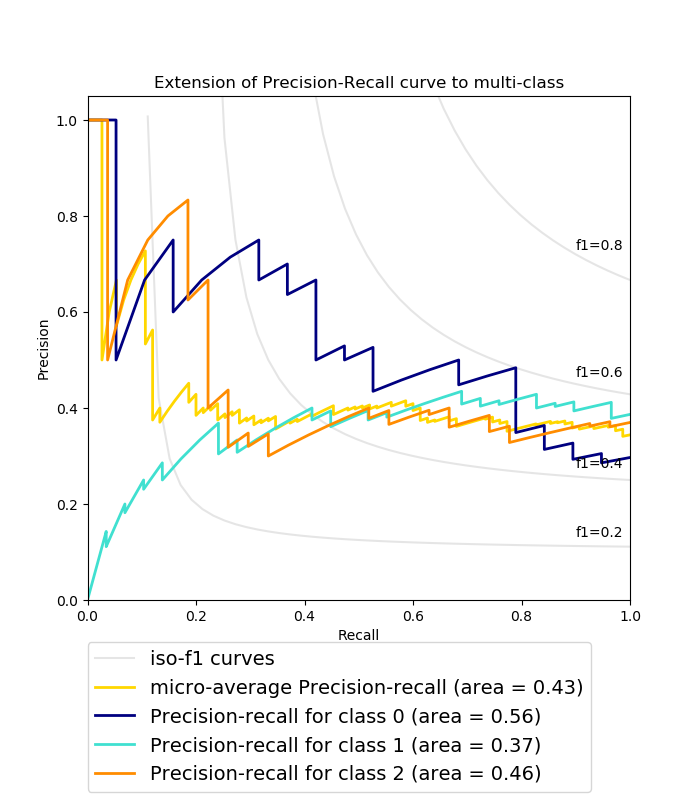
Figure: PR Curves, from scikit-learn
The figure above shows some example PR curves. The AUPRC for a given class is simply the area beneath its PR curve.
It’s a bit trickier to interpret AUPRC than it is to interpret AUROC (the area under the receiver operating characteristic). That’s because the baseline for AUROC is always going to be 0.5 — a random classifier, or a coin toss, will get you an AUROC of 0.5. But with AUPRC, the baseline is equal to the fraction of positives (Saito et al.), where the fraction of positives is calculated as (# positive examples / total # examples). That means that different classes have different AUPRC baselines. A class with 12% positives has a baseline AUPRC of 0.12, so obtaining an AUPRC of 0.40 on this class is great. However a class with 98% positives has a baseline AUPRC of 0.98, which means that obtaining an AUPRC of 0.40 on this class is bad.
For many real-world data sets, particularly medical datasets, the fraction of positives is often less than 0.5, meaning that AUPRC has a lower baseline value than AUROC. The AUPRC is thus frequently smaller in absolute value than the AUROC. For example, it’s possible to obtain an AUROC of 0.8 and an AUPRC of 0.3. I think this is one reason that AUPRC isn’t reported as often as AUROC in the literature. It just “sounds more impressive” to obtain performance of 0.8, even though the more meaningful number of the problem at hand very well might be the 0.3 AUPRC. Don’t let trends discourage you; AUPRC is a critical metric to calculate in problems where properly classifying the positives is important – for example, predicting a patient’s diagnosis on the basis of a laboratory test, or predicting whether a patient will suffer complications, or predicting whether a patient will need to visit a hospital. You can always report the AUPRC and AUROC together.
How to Calculate AUPRC
The AUPRC is calculated as the area under the PR curve. A PR curve shows the trade-off between precision and recall across different decision thresholds.
(Note that “recall” is another name for the true positive rate (TPR). Thus, AUPRC and AUROC both make use of the TPR. For a review of TPR, precision, and decision thresholds, see Measuring Performance: The Confusion Matrix.)
The x-axis of a PR curve is the recall and the y-axis is the precision. This is in contrast to ROC curves, where the y-axis is the recall and the x-axis is FPR. Similar to plotted ROC curves, in a plotted PR curve the decision thresholds are implicit and are not shown as a separate axis.
- Often, a PR curve starts at the upper left corner, i.e. the point (recall = 0, precision = 1) which corresponds to a decision threshold of 1 (where every example is classified as negative, because all predicted probabilities are less than 1). In more detail, when the example with the largest predicted output value is indeed truly positive (its ground truth is 1), then the PR curve starts at (recall = 0, precision = 1). In these situations, the model did a good job assigning the largest predicted output value to an example that is indeed positive.
- However, if the example with the largest predicted output value is actually negative (its ground truth is 0), then the PR curve will instead intersect with the point (recall = 0, precision = 0). In other words, if the model unfortunately produced a large predicted output value for something that is actually negative, that changes the starting point of the PR curve. Thus the ground truth label of the example with the largest output value has a big effect on the appearance of the PR curve. For more detail, see Boyd et al. (And thank you to an astute reader, Dr. W, for pointing out this phenomenon!)
- A PR curve ends at the lower right, where recall = 1 and precision is low. This corresponds to a decision threshold of 0 (where every example is classified as positive, because all predicted probabilities are greater than 0.) Note that estimates of precision for recall near zero tend to have high variance.
- The points in between, which create the PR curve, are obtained by calculating the precision and recall for different decision thresholds between 1 and 0. For a rough “angular” curve you would use only a few decision thresholds. For a smoother curve, you would use many decision thresholds.
Why do we look at the trade-off between precision and recall? It’s important to consider both recall and precision together, because you could achieve perfect recall (but bad precision) using a naive classifier that marked everything positive, and you could achieve perfect precision (but bad recall) using a naive classifier that marked everything negative.
To calculate AUPRC, we calculate the area under the PR curve. There are multiple methods for calculation of the area under the PR curve, including the lower trapezoid estimator, the interpolated median estimator, and the average precision.
I like to use average precision to calculate AUPRC. In Python, average precision is calculated as follows:
import sklearn.metrics

auprc = sklearn.metrics.average_precision_score(true_labels, predicted_probs)
For this function you provide a vector of the ground truth labels (true_labels) and a vector of the corresponding predicted probabilities from your model (predicted_probs.) Sklearn will use this information to calculate the average precision for you.
From the function documentation, the average precision “summarizes a precision-recall curve as the weighted mean of precisions achieved at each threshold, with the increase in recall from the previous threshold used as the weight. […] This implementation is not interpolated and is different from outputting the area under the precision-recall curve with the trapezoidal rule, which uses linear interpolation and can be too optimistic.”
Additional Section Reference: Boyd et al., “Area Under the Precision-Recall Curve: Point Estimates and Confidence Intervals.”
AUPRC & True Negatives
One interesting feature of PR curves is that they do not use true negatives at all:
- Recall = TPR = True Positives / (True Positives + False Negatives). Recall can be thought of as the ability of the classifier to correctly mark all positive examples as positive.
- Precision = True Positives / (True Positives + False Positives). Precision can be thought of as the ability of the classifier not to wrongly label a negative sample as positive (ref)
Because PR curves don’t use true negatives anywhere, the AUPRC won’t be “swamped” by a large proportion of true negatives in the data. You can use AUPRC on a dataset with 98% negative/2% positive examples, and it will “focus” on how the model handles the 2% positive examples. If the model handles the positive examples well, AUPRC will be high. If the model does poorly on the positive examples, AUPRC will be low.
Ironically, AUPRC can often be most useful when its baseline is lowest, because there are many datasets with large numbers of true negatives in which the goal is to handle the small fraction of positives as best as possible.
What if my model predicts more than two classes?
If your model predicts multiple classes, then you can pretend your task is composed of many different binary classification tasks, and calculate average precision for Class A vs. Not Class A, Class B vs. Not Class B, Class C vs. Not Class C…etc.
Summary
- There are many ways to calculate AUPRC, including average precision.
- A model achieves perfect AUPRC when it finds all the positive examples (perfect recall) without accidentally marking any negative examples as positive (perfect precision).
- The baseline of AUPRC is equal to the fraction of positives. If a dataset consists of 8% cancer examples and 92% healthy examples, the baseline AUPRC is 0.08, so obtaining an AUPRC of 0.40 in this scenario is good!
- AUPRC is most useful when you care a lot about your model handling the positive examples correctly.
- The calculation for AUPRC does not involve true negatives at all.
About the Featured Image
The featured image of the balance is modified from here.
Want to be the first to hear about my articles bridging healthcare, artificial intelligence, and business—and get a free list of my favorite health AI resources? Sign up here.

Comments are closed.